项目概述
这是一个基于Streamlit的交互式K-means聚类学习平台,让用户能够从零开始理解并实践K-means算法。项目包含了数据生成、算法演示、K值选择、实际应用和交互学习等多个模块。
技术栈
-
前端/界面: Streamlit
-
数据处理: NumPy, Pandas
-
机器学习: Scikit-learn
-
可视化: Matplotlib, Plotly, Seaborn
-
图像处理: PIL (Pillow)
代码功能逐段解析
第一部分:导入库
python
import streamlit as st
import numpy as np
import pandas as pd
import matplotlib.pyplot as plt
import plotly.express as px
import plotly.graph_objects as go
from sklearn.cluster import KMeans
from sklearn.metrics import silhouette_score
from sklearn.datasets import make_blobs
from sklearn.preprocessing import StandardScaler
import seaborn as sns
from io import StringIO
from PIL import Image
import time
import base64
from matplotlib.colors import ListedColormap
import warnings
这部分代码导入了项目所需的所有Python库。Streamlit用于构建Web应用界面;NumPy和Pandas用于数值计算和数据处理;Matplotlib、Plotly和Seaborn用于数据可视化;Scikit-learn提供机器学习算法(K-means等);PIL处理图像;其他库用于辅助功能如数据编码、时间处理等。
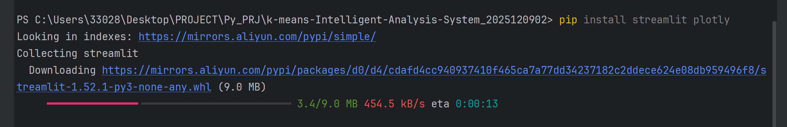
下载相关的库:
第二部分:设置中文字体和警告
python
plt.rcParams['font.sans-serif'] = ['SimHei', 'Microsoft YaHei', 'DejaVu Sans']
plt.rcParams['axes.unicode_minus'] = False
warnings.filterwarnings('ignore')这段代码配置Matplotlib以支持中文显示,设置了中文字体列表,确保图表中的中文能够正确渲染,同时禁用了负号显示问题。warnings.filterwarnings('ignore')用于抑制警告信息,保持界面整洁。
第三部分:设置Streamlit页面配置
python
st.set_page_config(
    page_title="K-means智能客户分群与可视化分析系统",
    page_icon="📊",
    layout="wide"
)这段代码配置Streamlit应用的页面属性,包括页面标题、图标和布局方式。"📊"是页面图标emoji,layout="wide"表示使用宽屏布局,使应用在浏览器中占据更宽的空间。
第四部分:标题和介绍
python
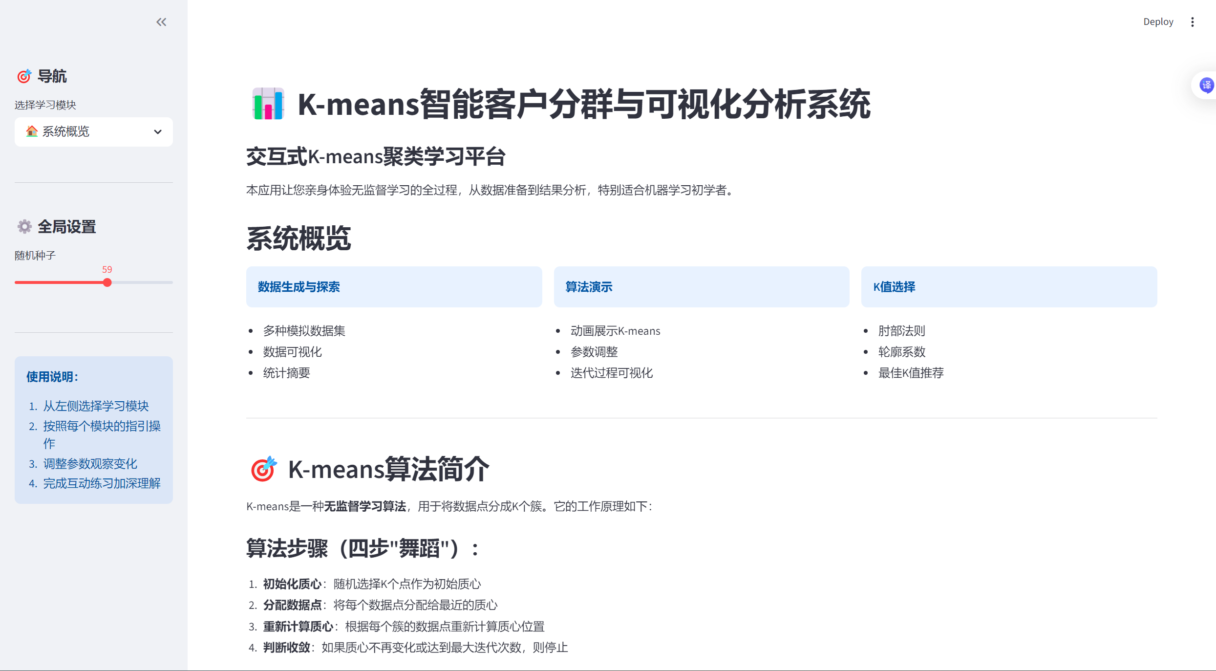
st.title("📊 K-means智能客户分群与可视化分析系统")
st.markdown("""
### 交互式K-means聚类学习平台
本应用让您亲身体验无监督学习的全过程,从数据准备到结果分析,特别适合机器学习初学者。
""")这段代码在应用主区域显示标题和介绍文字。st.title()显示主标题,st.markdown()支持Markdown格式文本,用于创建格式化的介绍内容,说明应用的目的和适用人群。
第五部分:创建侧边栏
python
with st.sidebar:
    st.header("🎯 导航")
    app_mode = st.selectbox(
        "选择学习模块",
        ["🏠 系统概览", "📈 数据生成与探索", "🔄 K-means算法演示",
         "🔍 K值选择助手", "🌐 实际应用场景", "🎓 交互式学习"]
    )

    st.markdown("---")
    st.header("⚙️ 全局设置")
    random_state = st.slider("随机种子", 0, 100, 42)
    np.random.seed(random_state)

    st.markdown("---")
    st.info("""
    **使用说明:**
    1. 从左侧选择学习模块
    2. 按照每个模块的指引操作
    3. 调整参数观察变化
    4. 完成互动练习加深理解
    """)
这段代码在页面左侧创建了一个侧边栏,包含导航菜单、全局设置和使用说明。用户可以通过下拉菜单选择不同模块,通过滑块设置随机种子(确保实验可重复性),并查看使用指南。
第六部分:系统概览模块
python
if app_mode == "🏠 系统概览":
    st.header("系统概览")

    col1, col2, col3 = st.columns(3)

    with col1:
        st.info("**数据生成与探索**")
        st.markdown("""
        - 多种模拟数据集
        - 数据可视化
        - 统计摘要
        """)

    with col2:
        st.info("**算法演示**")
        st.markdown("""
        - 动画展示K-means
        - 参数调整
        - 迭代过程可视化
        """)

    with col3:
        st.info("**K值选择**")
        st.markdown("""
        - 肘部法则
        - 轮廓系数
        - 最佳K值推荐
        """)

    st.markdown("---")

    # K-means算法解释
    st.header("🎯 K-means算法简介")

    st.markdown("""
    K-means是一种**无监督学习算法**,用于将数据点分成K个簇。它的工作原理如下:

    ### 算法步骤(四步"舞蹈"):

    1. **初始化质心**:随机选择K个点作为初始质心
    2. **分配数据点**:将每个数据点分配给最近的质心
    3. **重新计算质心**:根据每个簇的数据点重新计算质心位置
    4. **判断收敛**:如果质心不再变化或达到最大迭代次数,则停止

    ### 数学公式:

    **目标函数(惯量/簇内平方和)**:
    $$
    J = \sum_{i=1}^{K} \sum_{x \in C_i} \|x - \mu_i\|^2
    $$

    其中:
    - $K$: 聚类数量
    - $C_i$: 第i个簇
    - $\mu_i$: 第i个簇的质心
    - $x$: 数据点
    """)
当用户选择"系统概览"模块时,这段代码显示系统功能介绍、K-means算法详细解释和交互式示例。它创建了三个信息卡片展示主要功能,详细说明了算法原理和数学公式,并提供了一个可调节K值的实时聚类演示。
第七部分:数据生成函数模块
python
import numpy as np
import pandas as pd
from sklearn.datasets import make_blobs

def generate_customer_data(n_samples=300, n_clusters=3, noise_level=0.8, random_state=42):
    """
    生成模拟商场客户数据
    """
    centers = np.array([[5, 1], [1, 5], [3, 3], [7, 7]])[:n_clusters]
    X, true_labels = make_blobs(
        n_samples=n_samples,
        centers=centers,
        cluster_std=noise_level,
        random_state=random_state
    )

    # 调整数据范围使其更符合实际
    X[:, 0] = X[:, 0] * 10000 + 20000  # 年消费金额:2万-10万
    X[:, 1] = X[:, 1] * 500 + 500  # 单次消费金额:0-1000元

    df = pd.DataFrame(X, columns=['年消费金额(元)', '单次消费金额(元)'])
    df['客户类型'] = true_labels

    return df

def generate_pet_data(n_samples=300, n_clusters=3, noise_level=0.8, random_state=42):
    """
    生成宠物特征数据
    """
    centers = np.array([[1, 8], [5, 3], [8, 1], [3, 5]])[:n_clusters]
    X, true_labels = make_blobs(
        n_samples=n_samples,
        centers=centers,
        cluster_std=noise_level,
        random_state=random_state
    )

    # 调整数据范围
    X[:, 0] = X[:, 0] * 10 + 10  # 体型大小:10-100cm
    X[:, 1] = X[:, 1] * 100 + 200  # 叫声频率:100-1000Hz

    df = pd.DataFrame(X, columns=['体型大小(cm)', '叫声频率(Hz)'])
    df['宠物类型'] = true_labels

    return df

def generate_student_data(n_samples=300, n_clusters=3, noise_level=0.8, random_state=42):
    """
    生成学生行为数据
    """
    centers = np.array([[2, 6], [4, 8], [6, 4], [8, 9]])[:n_clusters]
    X, true_labels = make_blobs(
        n_samples=n_samples,
        centers=centers,
        cluster_std=noise_level,
        random_state=random_state
    )

    # 调整数据范围
    X[:, 0] = X[:, 0] * 5 + 10  # 学习时间:10-50小时/周
    X[:, 1] = X[:, 1] * 10 + 60  # 考试成绩:60-100分

    df = pd.DataFrame(X, columns=['学习时间(小时/周)', '考试成绩(分)'])
    df['学生类型'] = true_labels

    return df
这些函数专门用于生成不同类型的模拟数据集。每个函数都使用Scikit-learn的make_blobs生成具有指定簇数、样本量和噪声水平的数据,然后将数据转换为实际业务场景下的数值范围(如年消费金额、考试成绩等),以便更贴近实际应用。
第八部分:K-means算法演示类
python
import numpy as np
import matplotlib.pyplot as plt
from sklearn.cluster import KMeans
from sklearn.decomposition import PCA

class KMeansVisualizer:
    def __init__(self, random_state=42):
        self.random_state = random_state

    def create_step_by_step_animation(self, X, k=3, max_iter=10, init_method='k-means++'):
        """
        创建分步K-means演示动画
        """
        # 如果数据维度高,使用PCA降维
        if X.shape[1] > 2:
            pca = PCA(n_components=2)
            X_vis = pca.fit_transform(X)
        else:
            X_vis = X

        # 初始化K-means
        kmeans = KMeans(
            n_clusters=k,
            init=init_method,
            max_iter=1,
            n_init=1,
            random_state=self.random_state
        )

        centroids_history = []
        labels_history = []

        for i in range(max_iter):
            if i == 0:
                kmeans.fit(X_vis)
            else:
                kmeans.max_iter = i + 1
                kmeans.fit(X_vis)

            centroids_history.append(kmeans.cluster_centers_.copy())
            labels_history.append(kmeans.labels_.copy())

        return X_vis, centroids_history, labels_history

    def plot_iteration(self, X, centroids, labels, iteration):
        """
        绘制单次迭代结果
        """
        k = len(centroids)
        fig, ax = plt.subplots(figsize=(10, 7))

        # 绘制数据点
        colors = plt.cm.tab10(np.arange(k) / max(k, 1))
        for cluster_id in range(k):
            cluster_points = X[labels == cluster_id]
            ax.scatter(
                cluster_points[:, 0], cluster_points[:, 1],
                color=colors[cluster_id], alpha=0.6,
                edgecolors='black', linewidth=0.5,
                label=f'簇 {cluster_id + 1}'
            )

        # 绘制质心
        ax.scatter(
            centroids[:, 0], centroids[:, 1],
            marker='*', s=400, c='red', edgecolors='black',
            linewidth=1.5, label='质心'
        )

        ax.set_title(f'K-means聚类 (K={k}) - 迭代 {iteration}')
        ax.set_xlabel('特征1' if X.shape[1] == 2 else '主成分1')
        ax.set_ylabel('特征2' if X.shape[1] == 2 else '主成分2')
        ax.legend()
        ax.grid(True, alpha=0.3)

return fig这个类封装了K-means算法的可视化功能。create_step_by_step_animation方法实现了分步动画演示功能,包括数据降维(如果维度高)和记录每次迭代的质心位置;plot_iteration方法绘制单次迭代的可视化结果,用不同颜色区分簇,用星号标记质心。
第九部分:K值选择助手类
python
import numpy as np
import matplotlib.pyplot as plt
from sklearn.cluster import KMeans
from sklearn.metrics import silhouette_score

class KSelectionHelper:
    def __init__(self, random_state=42):
        self.random_state = random_state

    def calculate_metrics(self, X, k_range):
        """
        计算不同K值下的评估指标
        """
        inertias = []
        silhouette_scores = []
        models = []

        for k in k_range:
            # 训练K-means模型
            kmeans = KMeans(n_clusters=k, random_state=self.random_state)
            labels = kmeans.fit_predict(X)

            # 保存模型
            models.append(kmeans)

            # 计算惯量
            inertias.append(kmeans.inertia_)

            # 计算轮廓系数(需要至少2个簇)
            if k > 1:
                silhouette_scores.append(silhouette_score(X, labels))
            else:
                silhouette_scores.append(0)

        return inertias, silhouette_scores, models

    def plot_elbow_method(self, k_range, inertias):
        """
        绘制肘部法则图
        """
        fig, ax = plt.subplots(figsize=(10, 6))
        ax.plot(k_range, inertias, 'bo-', linewidth=2, markersize=8)
        ax.set_xlabel('聚类数量 (K)')
        ax.set_ylabel('惯量 (簇内平方和)')
        ax.set_title('肘部法则: 惯量随K值的变化')
        ax.grid(True, alpha=0.3)

        # 标记可能的肘点
        if len(inertias) >= 3:
            differences = np.diff(inertias)
            relative_differences = differences / inertias[:-1]
            diff_of_diffs = np.diff(relative_differences)

            if len(diff_of_diffs) > 0:
                elbow_index = np.argmax(diff_of_diffs) + 1
                if elbow_index < len(k_range):
                    elbow_k = list(k_range)[elbow_index]
                    ax.axvline(x=elbow_k, color='r', linestyle='--', alpha=0.7)
                    ax.text(elbow_k + 0.1, max(inertias) * 0.9,
                           f'建议K={elbow_k}', color='red', fontsize=12)

        return fig, elbow_k if 'elbow_k' in locals() else None

    def plot_silhouette_scores(self, k_range, silhouette_scores):
        """
        绘制轮廓系数图
        """
        fig, ax = plt.subplots(figsize=(10, 6))
        ax.plot(k_range, silhouette_scores, 'go-', linewidth=2, markersize=8)
        ax.set_xlabel('聚类数量 (K)')
        ax.set_ylabel('轮廓系数')
        ax.set_title('轮廓系数随K值的变化')
        ax.grid(True, alpha=0.3)

        # 标记最大轮廓系数
        if len(silhouette_scores) > 0:
            max_index = np.argmax(silhouette_scores)
            best_k = list(k_range)[max_index]
            best_score = silhouette_scores[max_index]

            ax.axvline(x=best_k, color='r', linestyle='--', alpha=0.7)
            ax.plot(best_k, best_score, 'ro', markersize=12)
            ax.text(best_k + 0.1, best_score,
                   f'最佳K={best_k} (分数={best_score:.3f})',
                   color='red', fontsize=12)

return fig, best_k if 'best_k' in locals() else None这个类帮助用户确定最佳K值。它计算不同K值下的评估指标(惯量和轮廓系数),plot_elbow_method方法绘制肘部法则图并自动检测"肘点",plot_silhouette_scores方法绘制轮廓系数图并标记最优K值,为K值选择提供数据支持。
第十部分:实际应用场景类
python
import numpy as np
import pandas as pd
import matplotlib.pyplot as plt
from sklearn.cluster import KMeans
from sklearn.preprocessing import StandardScaler
from PIL import Image
import base64
from io import BytesIO

class CustomerSegmentation:
    def __init__(self, random_state=42):
        self.random_state = random_state

    def generate_customer_data(self, n_customers=300, n_segments=3):
        """
        生成模拟客户数据用于细分分析
        """
        np.random.seed(self.random_state)

        # 创建不同群体的客户
        segments_centers = np.array([
            [80000, 800, 20, 30],  # VIP客户
            [30000, 300, 8, 90],  # 普通客户
            [10000, 100, 2, 180],  # 潜在流失客户
        ])[:n_segments]

        customer_data = []
        for i, center in enumerate(segments_centers):
            n_segment = n_customers // n_segments
            if i == n_segments - 1:
                n_segment = n_customers - (n_segments - 1) * (n_customers // n_segments)

            segment_data = np.random.normal(
                loc=center,
                scale=center * 0.2,
                size=(n_segment, 4)
            )
            customer_data.append(segment_data)

        customer_data = np.vstack(customer_data)
        customer_data = np.abs(customer_data)  # 确保数据为正数

        # 创建DataFrame
        df_customers = pd.DataFrame(customer_data, columns=[
            '年消费金额(元)', '单次消费金额(元)', '月购买频率', '最近购买(天前)'
        ])
        df_customers['客户ID'] = range(1, len(df_customers) + 1)

        return df_customers

    def analyze_segments(self, df_customers, n_clusters=3):
        """
        执行客户细分分析
        """
        # 选择用于聚类的特征
        features = ['年消费金额(元)', '单次消费金额(元)', '月购买频率', '最近购买(天前)']
        X = df_customers[features].values

        # 标准化数据
        scaler = StandardScaler()
        X_scaled = scaler.fit_transform(X)

        # 使用K-means聚类
        kmeans = KMeans(n_clusters=n_clusters, random_state=self.random_state)
        df_customers['客户群体'] = kmeans.fit_predict(X_scaled)

        return df_customers, kmeans, X_scaled

class ImageColorQuantizer:
    def __init__(self, random_state=42):
        self.random_state = random_state

    def quantize_image(self, image, n_colors=16):
        """
        使用K-means减少图像颜色数量
        """
        # 将图像转换为numpy数组
        img_array = np.array(image)

        # 获取图像尺寸
        height, width = img_array.shape[:2]

        # 将图像重塑为2D数组 (像素 x RGB)
        if len(img_array.shape) == 3:
            img_reshaped = img_array.reshape(-1, 3)
        else:
            img_reshaped = img_array.reshape(-1, 1)

        # 使用K-means进行颜色量化
        kmeans = KMeans(n_clusters=n_colors, random_state=self.random_state)
        labels = kmeans.fit_predict(img_reshaped)

        # 用质心颜色替换每个像素的颜色
        quantized_colors = kmeans.cluster_centers_.astype(int)
        quantized_img = quantized_colors[labels].reshape(img_array.shape)

        return quantized_img, quantized_colors
这些类实现了K-means在不同领域的应用。CustomerSegmentation类生成模拟客户数据并执行细分分析;ImageColorQuantizer类使用K-means进行图像颜色量化,将图像颜色减少到指定数量,实现图像压缩效果。
第十一部分:交互式学习类
python
import streamlit as st
import numpy as np
import matplotlib.pyplot as plt
from sklearn.cluster import KMeans
from sklearn.datasets import make_blobs

class InteractiveLearning:
    def __init__(self, random_state=42):
        self.random_state = random_state

    def concept_quiz(self):
        """
        概念选择题
        """
        st.subheader("概念选择题")
        st.markdown("测试您对K-means算法的理解。")

        # 问题1
        st.markdown("### 问题 1: 什么是质心(centroid)?")

        answer1 = st.radio(
            "选择正确答案:",
            ["A. 数据集中最中间的点",
             "B. 一个簇中所有数据点的平均值",
             "C. 离所有点最近的数据点",
             "D. 数据集中最大值和最小值的中间点"],
            key="q1"
        )

        if st.button("检查答案1"):
            if answer1 == "B. 一个簇中所有数据点的平均值":
                st.success("✅ 正确!质心是一个簇中所有数据点的平均值(均值点)。")
            else:
                st.error("❌ 不正确。质心是一个簇中所有数据点的平均值。")

        return answer1

    def prediction_game(self):
        """
        预测游戏:预测新数据点的簇标签
        """
        st.subheader("预测游戏")
        st.markdown("### 预测新数据点的簇标签")

        # 生成聚类数据
        n_clusters = 3
        X, true_labels = make_blobs(
            n_samples=100,
            centers=n_clusters,
            cluster_std=0.8,
            random_state=self.random_state
        )

        # 训练K-means模型
        kmeans = KMeans(n_clusters=n_clusters, random_state=self.random_state)
        kmeans.fit(X)

        # 显示现有聚类
        fig, ax = plt.subplots(figsize=(8, 6))

        colors = plt.cm.tab10(np.arange(n_clusters) / max(n_clusters, 1))
        for i in range(n_clusters):
            cluster_points = X[kmeans.labels_ == i]
            ax.scatter(
                cluster_points[:, 0], cluster_points[:, 1],
                color=colors[i], alpha=0.7, edgecolors='black',
                linewidth=0.5, label=f'簇 {i + 1}'
            )

        # 绘制质心
        ax.scatter(
            kmeans.cluster_centers_[:, 0], kmeans.cluster_centers_[:, 1],
            marker='*', s=200, c='red', edgecolors='black',
            linewidth=1, label='质心'
        )

        ax.set_xlabel('特征1')
        ax.set_ylabel('特征2')
        ax.set_title('现有聚类')
        ax.legend()
        ax.grid(True, alpha=0.3)

        st.pyplot(fig)

return kmeans, X这个类创建了多种交互式学习活动。concept_quiz方法包含选择题测试用户对K-means概念的理解;prediction_game方法让用户预测新数据点的簇标签,并提供即时反馈和解释,帮助用户在游戏中学习。
第十二部分:页脚和学习资源
python
# 页脚
st.markdown("---")
st.markdown("""
### 📚 学习资源
- [Scikit-learn官方文档 - K-means](https://scikit-learn.org/stable/modules/clustering.html#k-means)
- [Towards Data Science - K-means详解](https://towardsdatascience.com/k-means-clustering-algorithm-applications-evaluation-methods-and-drawbacks-aa03e644b48a)
- [Stanford CS229 - K-means讲义](http://cs229.stanford.edu/notes/cs229-notes7a.pdf)

### 💡 提示
- 尝试调整不同参数观察效果变化
- 在实际数据集上练习K-means应用
- 理解算法的局限性,知道何时不使用K-means
""")

st.caption("© 2023 K-means智能客户分群与可视化分析系统 | 为机器学习初学者设计")
这段代码在页面底部显示学习资源和提示信息,包括相关文档链接和实用建议。这些资源帮助用户进一步深入学习K-means算法和相关知识,提升学习效果。
总结
整个项目通过模块化设计将复杂的K-means学习系统分解为多个功能单一、易于理解的组件。从环境配置到算法演示,从理论讲解到实践应用,每个部分都有明确职责,共同构成了一个完整的学习平台,适合不同基础的用户循序渐进地学习和实践K-means聚类算法。
如何创建和使用 run_app.bat
步骤 1: 创建批处理文件
-
打开项目文件夹:
- 导航到你的项目目录:
-
创建批处理文件:
-
在文件夹空白处右键 → 新建 → 文本文档
-
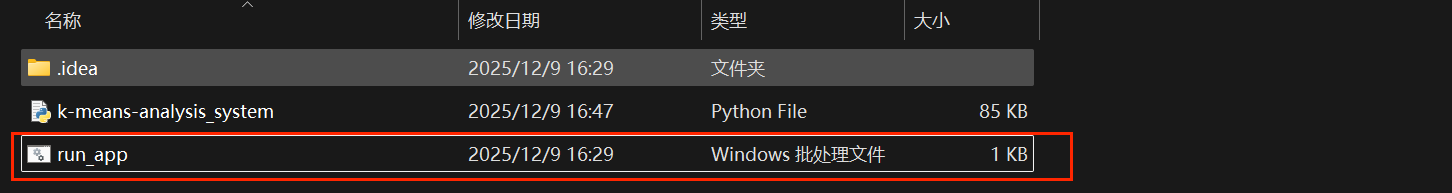
将新文件命名为
run_app.bat(注意:扩展名必须是.bat,不是.txt)
-
如果看不到文件扩展名:
- 打开任意文件夹 → 点击"查看"选项卡 → 勾选"文件扩展名"
-
编辑批处理文件内容:
-
右键点击
run_app.bat→ 选择"编辑"或"用记事本打开" -
输入以下代码:
-
python
@echo off
streamlit run "C:\Users\33028\Desktop\PROJECT\Py_PRJ\k-means-Intelligent-Analysis-System_2025120902\k-means-analysis_system.py"
pause
解释:
python
"C:\Users\33028\Desktop\PROJECT\Py_PRJ\k-means-Intelligent-Analysis-System_2025120902\k-means-analysis_system.py"对于这个,我们换成我们自己当前的目录即可
步骤 2: 使用批处理文件
-
双击运行:
- 找到
run_app.bat文件
- 找到
-
-
双击运行它
-
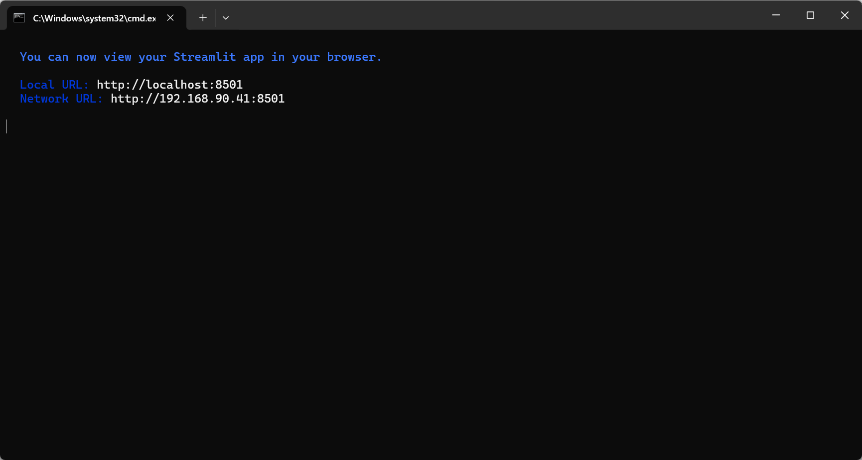
会弹出一个黑色命令行窗口(如下为第二次运行后的黑色命令行窗口)
-
-
第一次运行会发生什么:
-
如果这是第一次运行,它会自动安装所需的Python包
-
安装完成后会自动启动Streamlit应用
-
默认会自动打开浏览器访问
http://localhost:8501
-
-
正常运行效果:
- 命令行窗口会显示类似这样的信息:

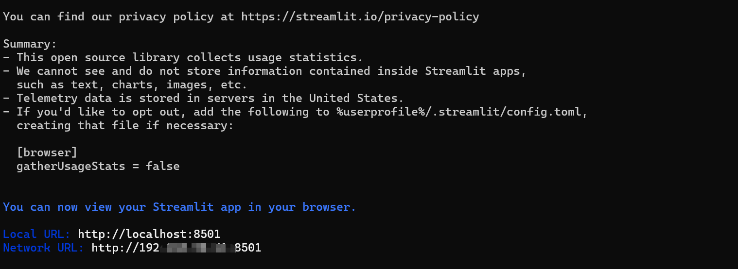
太好了!现在Streamlit已经成功启动了。你看到的这个提示是Streamlit的欢迎信息,询问你是否愿意接收他们的邮件通知。这个提示只会在第一次运行Streamlit时出现。
如何继续
1. 跳过邮箱提示(推荐)
直接按 Enter(回车)键,留空不填任何邮箱,然后按回车。这样就不会注册他们的邮件列表,可以直接进入你的应用。
2. 如果想接收Streamlit的邮件
输入你的邮箱地址,然后按回车。但通常对于学习项目,直接跳过就可以了。
接下来的步骤
输入邮箱(或留空按回车)后,你会看到类似这样的信息:
最终打开了下面这样的界面:
如何访问你的K-means应用
方法1:自动打开(通常会发生)
-
Streamlit会自动在你的默认浏览器中打开应用
-
浏览器会访问
http://localhost:8501
方法2:手动打开浏览器
如果浏览器没有自动打开:
-
打开Chrome、Edge、Firefox等浏览器
-
在地址栏输入:
http://localhost:8501 -
按回车
方法3:使用网络地址
如果你想让同一网络中的其他设备访问:
-
查看命令行中显示的"Network URL"(类似
http://192.168.1.100:8501) -
在其他设备的浏览器中输入这个地址
常见问题解决
问题1:浏览器没有自动打开
-
手动输入
http://localhost:8501 -
或者输入
http://127.0.0.1:8501
问题2:端口被占用
如果看到错误提示端口8501已被占用:
bash
streamlit run k-means-analysis_system.py --server.port 8502然后在浏览器访问 http://localhost:8502
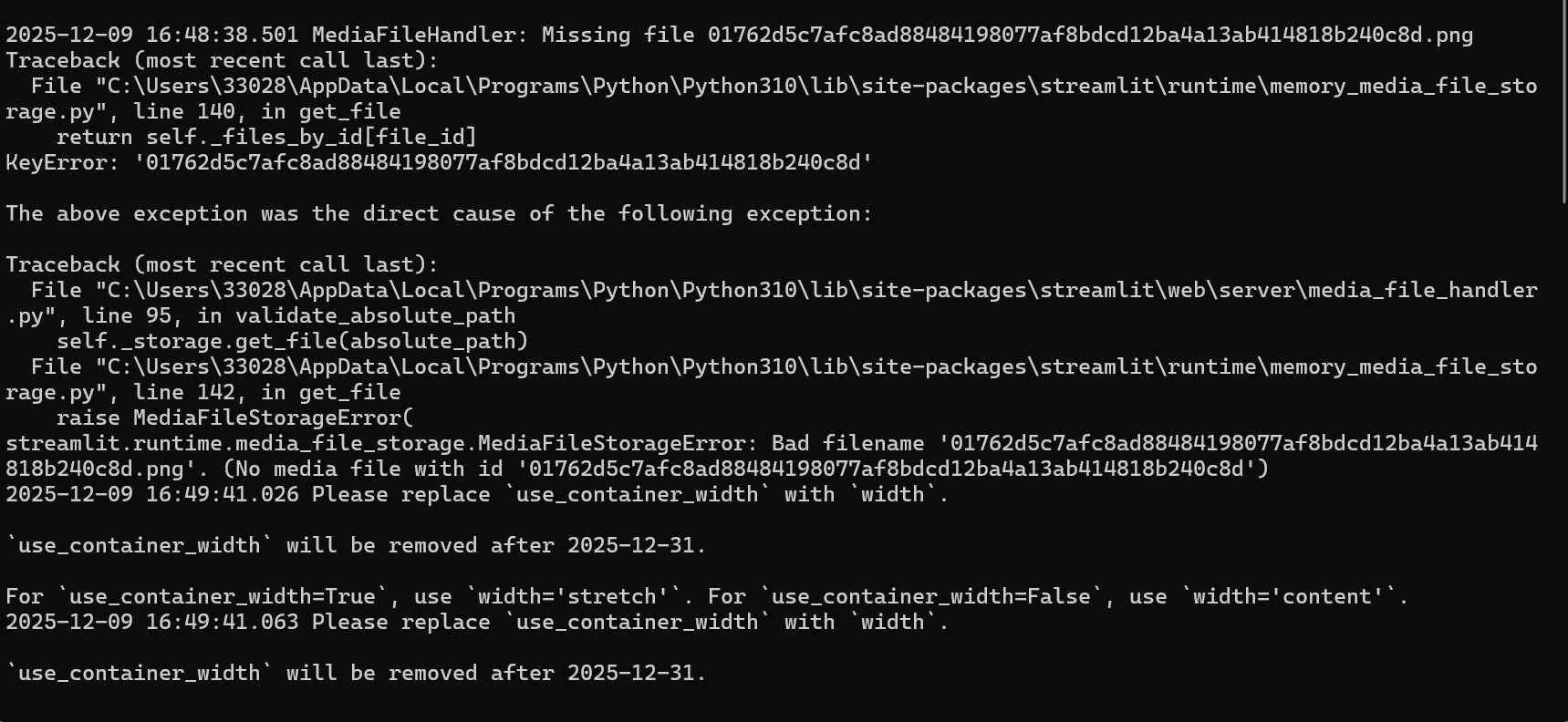
问题3:应用启动失败
检查命令行窗口中的错误信息,可能需要:
-
确保所有依赖包已安装
-
检查Python版本(需要Python 3.7+)
-
确保没有语法错误
使用应用的小技巧
一旦应用在浏览器中打开:
侧边栏导航 :左侧可以选择不同模块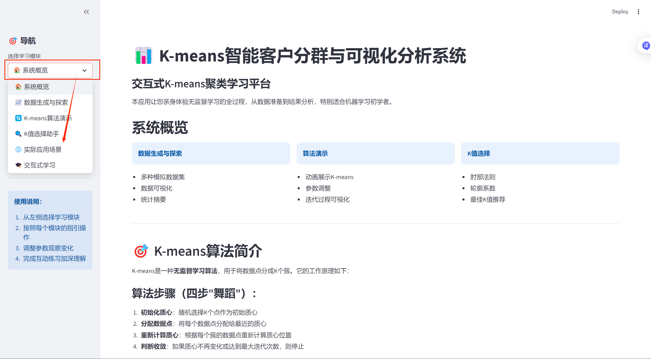
-
交互操作:
- 调整滑块改变参数
-
- 点击按钮运行算法
-
- 查看实时可视化效果
-
多页面功能:
- 数据生成与探索
-
- K-means算法演示
-
- K值选择助手
-
- 实际应用场景
-
- 交互式学习

- 响应式设计:应用会自动适应不同屏幕大小
我们的黑框中会根据我们的操作做出相应的反应:
如何停止应用
-
在命令行窗口 :按
Ctrl + C -
在浏览器中:点击右上角的菜单 → "Stop"
-
关闭命令行窗口:但建议先按Ctrl+C停止应用
项目完整源代码
python
import streamlit as st
import numpy as np
import pandas as pd
import matplotlib.pyplot as plt
import plotly.express as px
import plotly.graph_objects as go
from sklearn.cluster import KMeans
from sklearn.metrics import silhouette_score
from sklearn.datasets import make_blobs
from sklearn.preprocessing import StandardScaler
import seaborn as sns
from io import StringIO
from PIL import Image
import time
import base64
from matplotlib.colors import ListedColormap
import warnings
# 设置中文字体(如果需要显示中文)
plt.rcParams['font.sans-serif'] = ['SimHei', 'Microsoft YaHei', 'DejaVu Sans']
plt.rcParams['axes.unicode_minus'] = False
warnings.filterwarnings('ignore')
# 设置页面
st.set_page_config(
page_title="K-means智能客户分群与可视化分析系统",
page_icon="📊",
layout="wide"
)
# 标题和介绍
st.title("📊 K-means智能客户分群与可视化分析系统")
st.markdown("""
### 交互式K-means聚类学习平台
本应用让您亲身体验无监督学习的全过程,从数据准备到结果分析,特别适合机器学习初学者。
""")
# 创建侧边栏
with st.sidebar:
st.header("🎯 导航")
app_mode = st.selectbox(
"选择学习模块",
["🏠 系统概览", "📈 数据生成与探索", "🔄 K-means算法演示",
"🔍 K值选择助手", "🌐 实际应用场景", "🎓 交互式学习"]
)
st.markdown("---")
st.header("⚙️ 全局设置")
random_state = st.slider("随机种子", 0, 100, 42)
np.random.seed(random_state)
st.markdown("---")
st.info("""
**使用说明:**
1. 从左侧选择学习模块
2. 按照每个模块的指引操作
3. 调整参数观察变化
4. 完成互动练习加深理解
""")
# ==================== 系统概览模块 ====================
if app_mode == "🏠 系统概览":
st.header("系统概览")
col1, col2, col3 = st.columns(3)
with col1:
st.info("**数据生成与探索**")
st.markdown("""
- 多种模拟数据集
- 数据可视化
- 统计摘要
""")
with col2:
st.info("**算法演示**")
st.markdown("""
- 动画展示K-means
- 参数调整
- 迭代过程可视化
""")
with col3:
st.info("**K值选择**")
st.markdown("""
- 肘部法则
- 轮廓系数
- 最佳K值推荐
""")
st.markdown("---")
# K-means算法解释
st.header("🎯 K-means算法简介")
st.markdown("""
K-means是一种**无监督学习算法**,用于将数据点分成K个簇。它的工作原理如下:
### 算法步骤(四步"舞蹈"):
1. **初始化质心**:随机选择K个点作为初始质心
2. **分配数据点**:将每个数据点分配给最近的质心
3. **重新计算质心**:根据每个簇的数据点重新计算质心位置
4. **判断收敛**:如果质心不再变化或达到最大迭代次数,则停止
### 数学公式:
**目标函数(惯量/簇内平方和)**:
$$
J = \sum_{i=1}^{K} \sum_{x \in C_i} \|x - \mu_i\|^2
$$
其中:
- $K$: 聚类数量
- $C_i$: 第i个簇
- $\mu_i$: 第i个簇的质心
- $x$: 数据点
### 优点:
- 简单、高效、易于实现
- 对于球形簇效果很好
### 缺点:
- 需要预先指定K值
- 对初始质心敏感
- 对异常值敏感
- 假设簇是球形的
""")
# 添加一个简单的可视化示例
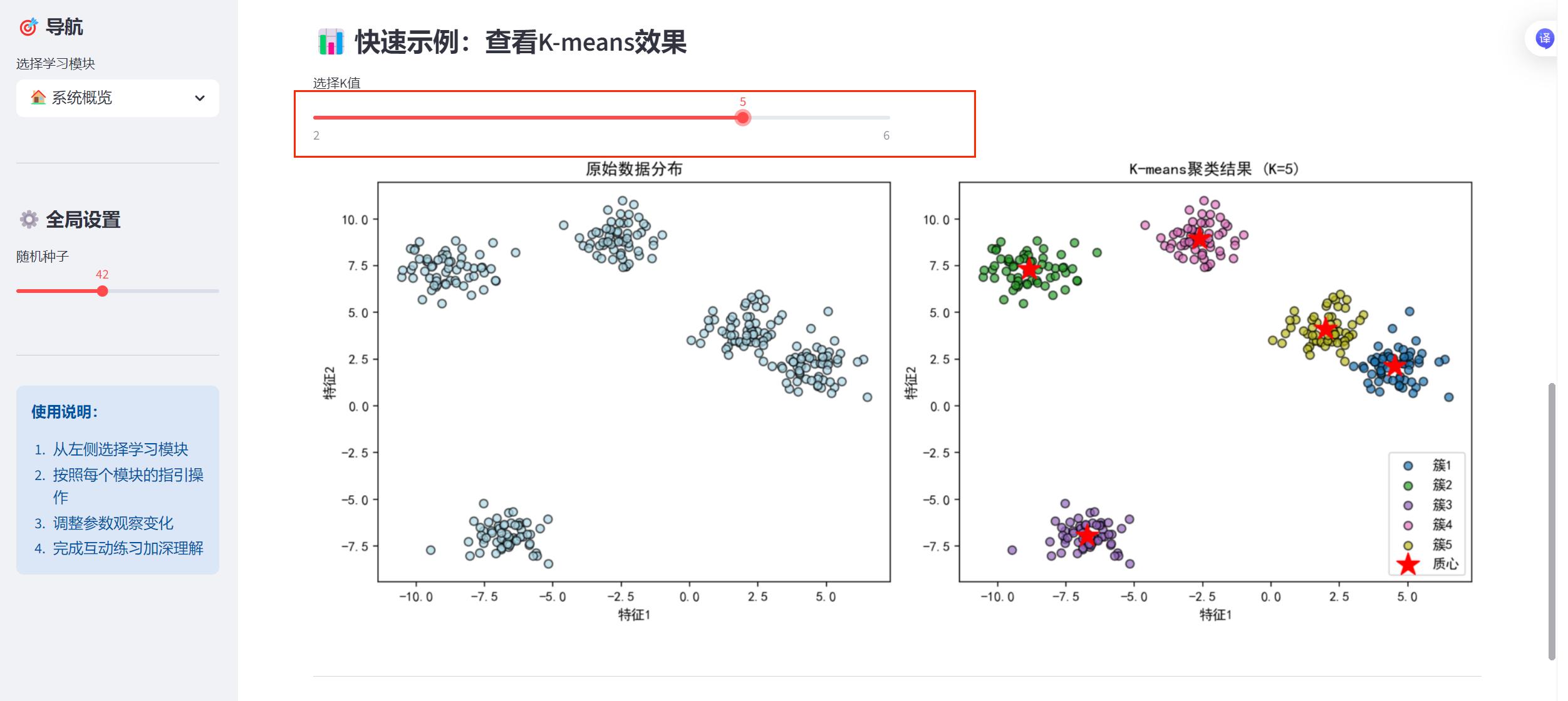
st.subheader("📊 快速示例:查看K-means效果")
col1, col2 = st.columns(2)
with col1:
example_k = st.slider("选择K值", 2, 6, 3)
# 生成示例数据
X, y = make_blobs(n_samples=300, centers=example_k,
cluster_std=0.8, random_state=random_state)
# 应用K-means
kmeans = KMeans(n_clusters=example_k, random_state=random_state)
labels = kmeans.fit_predict(X)
# 创建图表
fig, (ax1, ax2) = plt.subplots(1, 2, figsize=(12, 5))
# 原始数据
ax1.scatter(X[:, 0], X[:, 1], c='lightblue', edgecolors='black', alpha=0.7)
ax1.set_title('原始数据分布')
ax1.set_xlabel('特征1')
ax1.set_ylabel('特征2')
# 聚类结果
colors = plt.cm.tab10(np.arange(example_k) / max(example_k, 1))
for i in range(example_k):
ax2.scatter(X[labels == i, 0], X[labels == i, 1],
color=colors[i], edgecolors='black', alpha=0.7,
label=f'簇{i + 1}')
# 绘制质心
ax2.scatter(kmeans.cluster_centers_[:, 0],
kmeans.cluster_centers_[:, 1],
marker='*', s=300, c='red', label='质心')
ax2.set_title(f'K-means聚类结果 (K={example_k})')
ax2.set_xlabel('特征1')
ax2.set_ylabel('特征2')
ax2.legend()
plt.tight_layout()
st.pyplot(fig)
# ==================== 数据生成与探索模块 ====================
elif app_mode == "📈 数据生成与探索":
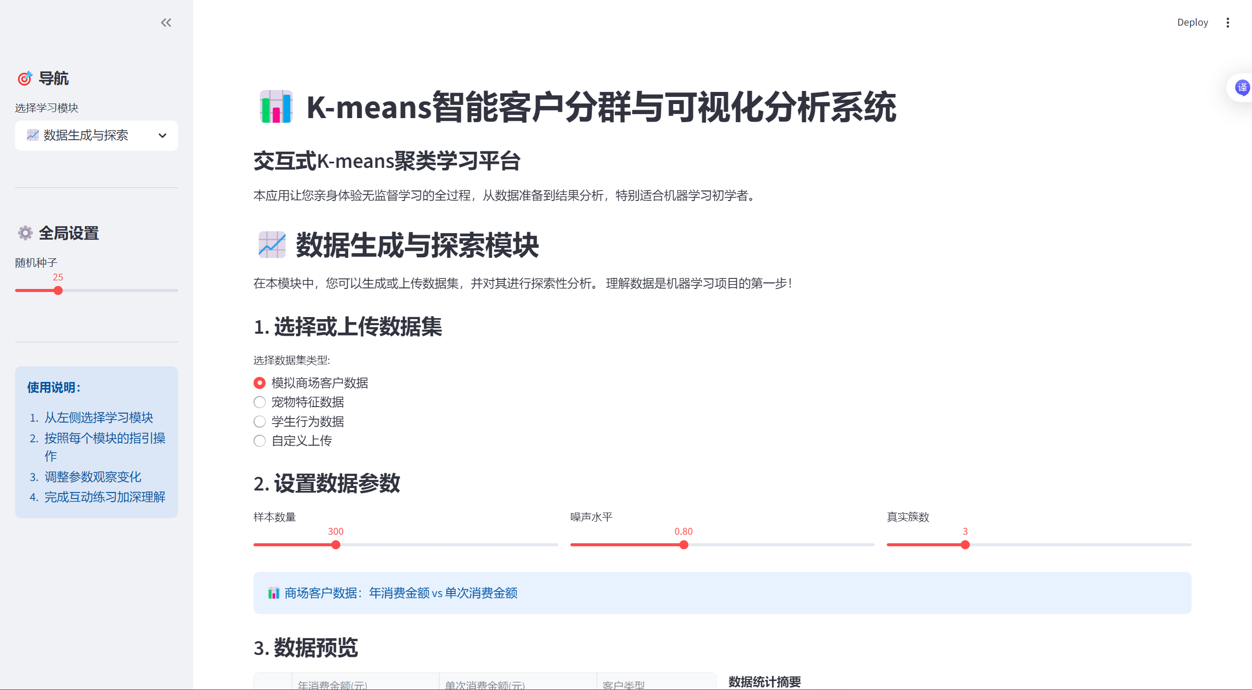
st.header("📈 数据生成与探索模块")
st.markdown("""
在本模块中,您可以生成或上传数据集,并对其进行探索性分析。
理解数据是机器学习项目的第一步!
""")
# 数据集选择
st.subheader("1. 选择或上传数据集")
dataset_option = st.radio(
"选择数据集类型:",
["模拟商场客户数据", "宠物特征数据", "学生行为数据", "自定义上传"]
)
# 数据生成参数
st.subheader("2. 设置数据参数")
col1, col2, col3 = st.columns(3)
with col1:
n_samples = st.slider("样本数量", 50, 1000, 300)
with col2:
noise_level = st.slider("噪声水平", 0.1, 2.0, 0.8, 0.1)
with col3:
n_clusters = st.slider("真实簇数", 2, 6, 3)
# 根据选择生成数据
if dataset_option == "模拟商场客户数据":
st.info("📊 商场客户数据:年消费金额 vs 单次消费金额")
# 生成模拟数据
centers = np.array([[5, 1], [1, 5], [3, 3], [7, 7]])[:n_clusters]
X, true_labels = make_blobs(n_samples=n_samples,
centers=centers,
cluster_std=noise_level,
random_state=random_state)
# 调整数据范围使其更符合实际
X[:, 0] = X[:, 0] * 10000 + 20000 # 年消费金额:2万-10万
X[:, 1] = X[:, 1] * 500 + 500 # 单次消费金额:0-1000元
df = pd.DataFrame(X, columns=['年消费金额(元)', '单次消费金额(元)'])
df['客户类型'] = true_labels
elif dataset_option == "宠物特征数据":
st.info("🐕 宠物特征数据:体型大小 vs 叫声频率")
# 生成模拟数据
centers = np.array([[1, 8], [5, 3], [8, 1], [3, 5]])[:n_clusters]
X, true_labels = make_blobs(n_samples=n_samples,
centers=centers,
cluster_std=noise_level,
random_state=random_state)
# 调整数据范围
X[:, 0] = X[:, 0] * 10 + 10 # 体型大小:10-100cm
X[:, 1] = X[:, 1] * 100 + 200 # 叫声频率:100-1000Hz
df = pd.DataFrame(X, columns=['体型大小(cm)', '叫声频率(Hz)'])
df['宠物类型'] = true_labels
elif dataset_option == "学生行为数据":
st.info("🎓 学生行为数据:学习时间 vs 考试成绩")
# 生成模拟数据
centers = np.array([[2, 6], [4, 8], [6, 4], [8, 9]])[:n_clusters]
X, true_labels = make_blobs(n_samples=n_samples,
centers=centers,
cluster_std=noise_level,
random_state=random_state)
# 调整数据范围
X[:, 0] = X[:, 0] * 5 + 10 # 学习时间:10-50小时/周
X[:, 1] = X[:, 1] * 10 + 60 # 考试成绩:60-100分
df = pd.DataFrame(X, columns=['学习时间(小时/周)', '考试成绩(分)'])
df['学生类型'] = true_labels
else: # 自定义上传
st.info("📁 上传您自己的数据集")
uploaded_file = st.file_uploader("选择CSV文件", type=['csv'])
if uploaded_file is not None:
df = pd.read_csv(uploaded_file)
st.success(f"成功上传数据集,包含 {df.shape[0]} 行和 {df.shape[1]} 列")
else:
# 提供示例数据
st.info("请上传CSV文件,或使用以下示例数据")
# 生成默认数据
X, true_labels = make_blobs(n_samples=n_samples,
n_features=2,
centers=n_clusters,
cluster_std=noise_level,
random_state=random_state)
df = pd.DataFrame(X, columns=['特征1', '特征2'])
df['真实标签'] = true_labels
# 显示数据
st.subheader("3. 数据预览")
col1, col2 = st.columns(2)
with col1:
st.dataframe(df.head(10), use_container_width=True)
with col2:
st.markdown("**数据统计摘要**")
st.dataframe(df.describe(), use_container_width=True)
# 数据可视化
st.subheader("4. 数据可视化")
# 选择可视化类型
viz_type = st.selectbox(
"选择可视化类型",
["散点图", "直方图", "箱线图", "相关热图"]
)
if viz_type == "散点图":
# 选择要绘制的列
numeric_cols = df.select_dtypes(include=[np.number]).columns.tolist()
if len(numeric_cols) >= 2:
col1, col2 = st.columns(2)
with col1:
x_col = st.selectbox("选择X轴特征", numeric_cols, index=0)
with col2:
y_col = st.selectbox("选择Y轴特征", numeric_cols, index=min(1, len(numeric_cols) - 1))
# 创建散点图
fig = px.scatter(df, x=x_col, y=y_col,
title=f"{x_col} vs {y_col}",
hover_data=df.columns.tolist())
st.plotly_chart(fig, use_container_width=True)
elif viz_type == "直方图":
numeric_cols = df.select_dtypes(include=[np.number]).columns.tolist()
if numeric_cols:
selected_col = st.selectbox("选择要可视化的特征", numeric_cols)
fig = px.histogram(df, x=selected_col,
title=f"{selected_col}的分布",
nbins=30)
st.plotly_chart(fig, use_container_width=True)
elif viz_type == "箱线图":
numeric_cols = df.select_dtypes(include=[np.number]).columns.tolist()
if numeric_cols:
selected_cols = st.multiselect("选择要可视化的特征", numeric_cols, default=numeric_cols[:3])
if selected_cols:
fig = px.box(df[selected_cols],
title="数据分布箱线图")
st.plotly_chart(fig, use_container_width=True)
elif viz_type == "相关热图":
numeric_cols = df.select_dtypes(include=[np.number]).columns.tolist()
if len(numeric_cols) > 1:
corr_matrix = df[numeric_cols].corr()
fig = px.imshow(corr_matrix,
text_auto=True,
aspect="auto",
title="特征相关热图",
color_continuous_scale='RdBu')
st.plotly_chart(fig, use_container_width=True)
# 保存数据以供后续使用
if 'current_data' not in st.session_state:
st.session_state.current_data = {}
st.session_state.current_data['X'] = df.select_dtypes(include=[np.number]).values
st.session_state.current_data['df'] = df
st.session_state.current_data['dataset_name'] = dataset_option
# ==================== K-means算法演示模块 ====================
elif app_mode == "🔄 K-means算法演示":
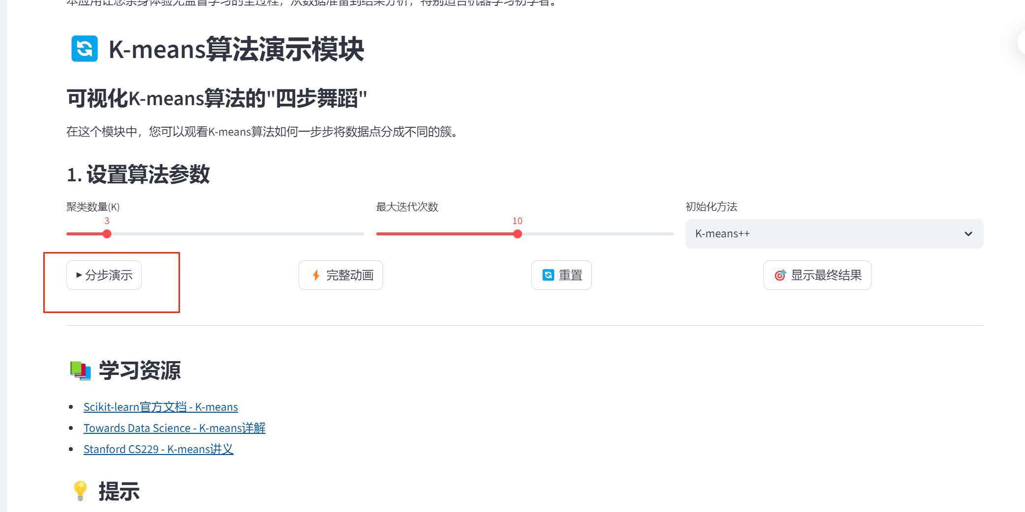
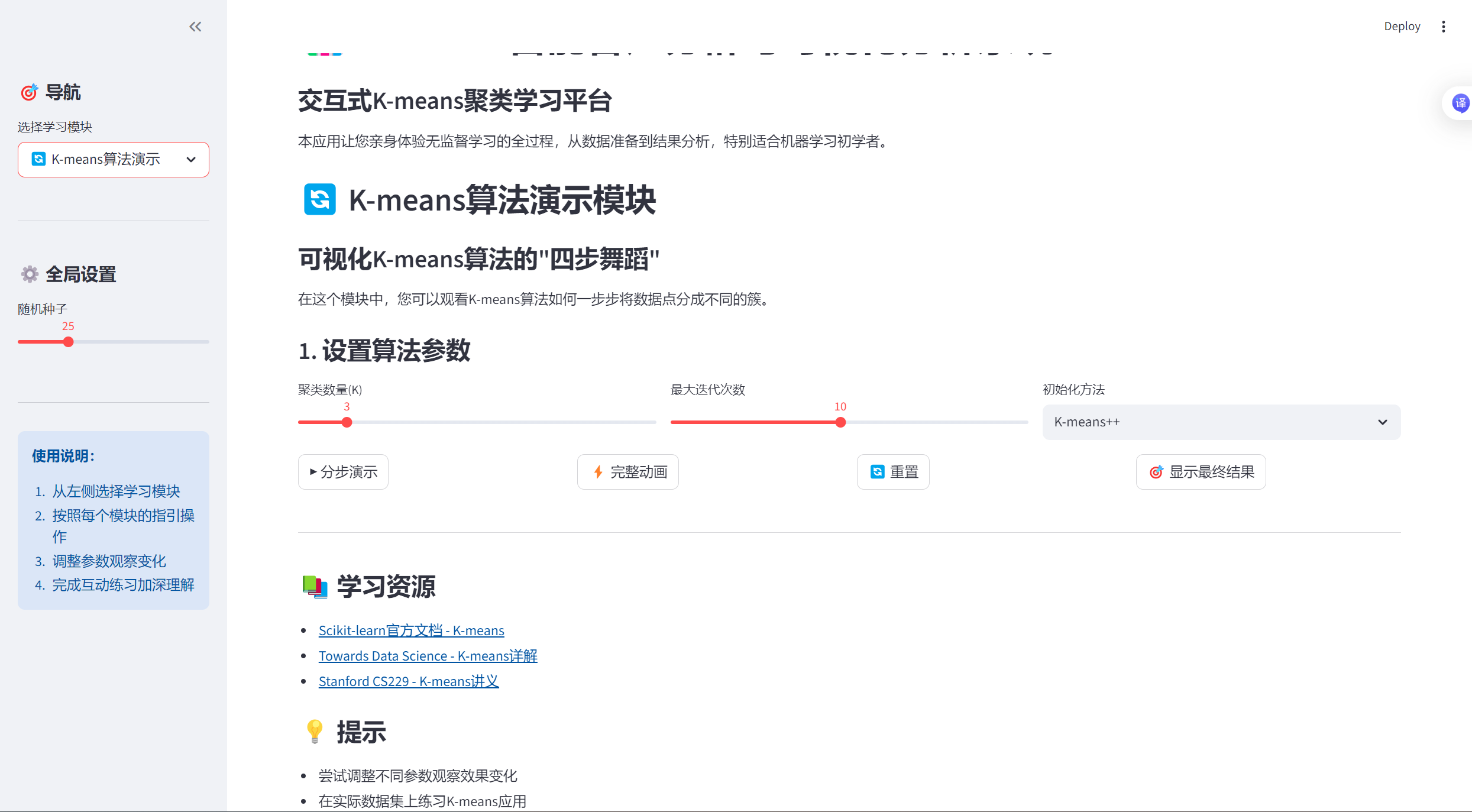
st.header("🔄 K-means算法演示模块")
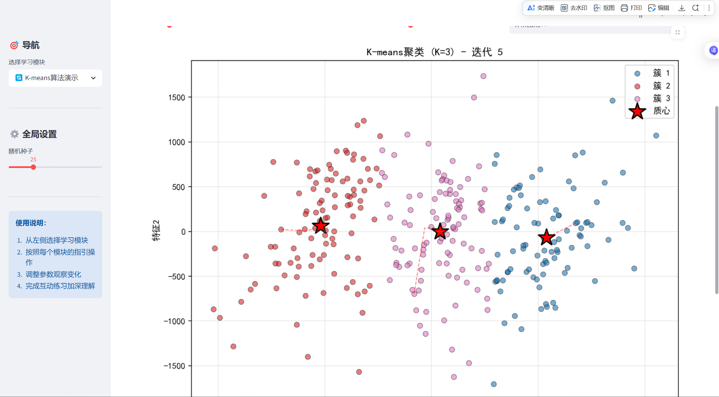
st.markdown("""
### 可视化K-means算法的"四步舞蹈"
在这个模块中,您可以观看K-means算法如何一步步将数据点分成不同的簇。
""")
# 检查是否有数据
if 'current_data' not in st.session_state or 'X' not in st.session_state.current_data:
st.warning("请先到'数据生成与探索'模块生成或上传数据。")
st.info("正在使用示例数据...")
X, _ = make_blobs(n_samples=300, centers=3, cluster_std=0.8, random_state=random_state)
df = pd.DataFrame(X, columns=['特征1', '特征2'])
else:
X = st.session_state.current_data['X']
df = st.session_state.current_data['df']
# 算法参数设置
st.subheader("1. 设置算法参数")
col1, col2, col3 = st.columns(3)
with col1:
k = st.slider("聚类数量(K)", 2, 10, 3)
with col2:
max_iter = st.slider("最大迭代次数", 1, 20, 10)
with col3:
init_method = st.selectbox(
"初始化方法",
["随机初始化", "K-means++"],
index=1
)
# 初始化方法映射
init_map = {"随机初始化": "random", "K-means++": "k-means++"}
# 创建用于动画的占位符
animation_placeholder = st.empty()
# 创建控制按钮
col1, col2, col3, col4 = st.columns(4)
with col1:
step_by_step = st.button("▶️ 分步演示")
with col2:
full_animation = st.button("⚡ 完整动画")
with col3:
reset_animation = st.button("🔄 重置")
with col4:
show_final = st.button("🎯 显示最终结果")
# 算法演示
if step_by_step or full_animation or show_final:
st.subheader("2. 算法演示过程")
# 准备数据
if X.shape[1] > 2:
# 使用PCA降维到2D以便可视化
from sklearn.decomposition import PCA
pca = PCA(n_components=2)
X_vis = pca.fit_transform(X)
st.info(f"数据从{X.shape[1]}维降维到2维以便可视化")
else:
X_vis = X
# 初始化K-means
kmeans = KMeans(n_clusters=k,
init=init_map[init_method],
max_iter=1 if step_by_step else max_iter,
n_init=1,
random_state=random_state)
# 用于存储每一步的结果
centroids_history = []
labels_history = []
# 执行算法
if step_by_step:
# 分步执行
progress_bar = st.progress(0)
status_text = st.empty()
for i in range(max_iter):
status_text.text(f"迭代 {i + 1}/{max_iter}")
if i == 0:
# 首次迭代:初始化质心
kmeans.fit(X_vis)
else:
# 后续迭代
kmeans.max_iter = i + 1
kmeans.fit(X_vis)
# 保存历史
centroids_history.append(kmeans.cluster_centers_.copy())
labels_history.append(kmeans.labels_.copy())
# 绘制当前状态
fig, ax = plt.subplots(figsize=(10, 7))
# 绘制数据点
colors = plt.cm.tab10(np.arange(k) / max(k, 1))
for cluster_id in range(k):
cluster_points = X_vis[labels_history[-1] == cluster_id]
ax.scatter(cluster_points[:, 0], cluster_points[:, 1],
color=colors[cluster_id], alpha=0.6,
edgecolors='black', linewidth=0.5,
label=f'簇 {cluster_id + 1}')
# 绘制质心
ax.scatter(centroids_history[-1][:, 0], centroids_history[-1][:, 1],
marker='*', s=400, c='red', edgecolors='black',
linewidth=1.5, label='质心')
# 绘制质心移动轨迹
if len(centroids_history) > 1:
for cluster_id in range(k):
# 获取该质心的历史位置
centroid_path = [step[cluster_id] for step in centroids_history]
centroid_path = np.array(centroid_path)
ax.plot(centroid_path[:, 0], centroid_path[:, 1],
'r--', alpha=0.5, linewidth=1)
ax.set_title(f'K-means聚类 (K={k}) - 迭代 {i + 1}')
ax.set_xlabel('特征1' if X_vis.shape[1] == 2 else '主成分1')
ax.set_ylabel('特征2' if X_vis.shape[1] == 2 else '主成分2')
ax.legend()
ax.grid(True, alpha=0.3)
animation_placeholder.pyplot(fig)
plt.close(fig)
# 更新进度
progress_bar.progress((i + 1) / max_iter)
# 如果是分步演示,等待用户点击
if step_by_step and i < max_iter - 1:
if not st.button(f"继续迭代 {i + 2}"):
break
elif full_animation:
# 完整动画
progress_bar = st.progress(0)
status_text = st.empty()
# 一次性训练
kmeans = KMeans(n_clusters=k,
init=init_map[init_method],
max_iter=max_iter,
n_init=1,
random_state=random_state)
kmeans.fit(X_vis)
# 为了动画,我们需要模拟每一步
# 创建一个自定义的K-means来记录历史
class KMeansWithHistory:
def __init__(self, n_clusters, init, max_iter, random_state):
self.n_clusters = n_clusters
self.init = init
self.max_iter = max_iter
self.random_state = random_state
def fit(self, X):
np.random.seed(self.random_state)
# 初始化质心
if self.init == 'k-means++':
# K-means++初始化
centroids = [X[np.random.randint(X.shape[0])]]
for _ in range(1, self.n_clusters):
distances = np.array([min([np.linalg.norm(x - c) ** 2 for c in centroids]) for x in X])
probabilities = distances / distances.sum()
cumulative_probabilities = probabilities.cumsum()
r = np.random.rand()
for j, p in enumerate(cumulative_probabilities):
if r < p:
centroids.append(X[j])
break
centroids = np.array(centroids)
else:
# 随机初始化
random_indices = np.random.choice(X.shape[0], self.n_clusters, replace=False)
centroids = X[random_indices]
self.centroids_history = [centroids.copy()]
self.labels_history = []
for iteration in range(self.max_iter):
# 步骤1: 分配标签
distances = np.sqrt(((X[:, np.newaxis, :] - centroids[np.newaxis, :, :]) ** 2).sum(axis=2))
labels = np.argmin(distances, axis=1)
self.labels_history.append(labels.copy())
# 步骤2: 更新质心
new_centroids = np.array([X[labels == i].mean(axis=0) for i in range(self.n_clusters)])
# 检查收敛
if np.allclose(centroids, new_centroids):
# 如果收敛,填充剩余的历史
for _ in range(iteration, self.max_iter):
self.labels_history.append(labels.copy())
self.centroids_history.append(new_centroids.copy())
break
centroids = new_centroids
self.centroids_history.append(centroids.copy())
self.cluster_centers_ = centroids
self.labels_ = labels
self.n_iter_ = iteration + 1
return self
# 使用自定义K-means
kmeans_custom = KMeansWithHistory(n_clusters=k,
init=init_map[init_method],
max_iter=max_iter,
random_state=random_state)
kmeans_custom.fit(X_vis)
# 动画显示
for i in range(len(kmeans_custom.centroids_history)):
status_text.text(f"迭代 {i + 1}/{max_iter}")
fig, ax = plt.subplots(figsize=(10, 7))
# 绘制数据点
if i < len(kmeans_custom.labels_history):
labels = kmeans_custom.labels_history[i]
else:
labels = kmeans_custom.labels_history[-1]
colors = plt.cm.tab10(np.arange(k) / max(k, 1))
for cluster_id in range(k):
cluster_points = X_vis[labels == cluster_id]
if len(cluster_points) > 0:
ax.scatter(cluster_points[:, 0], cluster_points[:, 1],
color=colors[cluster_id], alpha=0.6,
edgecolors='black', linewidth=0.5,
label=f'簇 {cluster_id + 1}')
# 绘制质心
centroids = kmeans_custom.centroids_history[i]
ax.scatter(centroids[:, 0], centroids[:, 1],
marker='*', s=400, c='red', edgecolors='black',
linewidth=1.5, label='质心')
# 绘制质心移动轨迹
if i > 0:
for cluster_id in range(k):
# 获取该质心的历史位置
centroid_path = np.array([step[cluster_id] for step in kmeans_custom.centroids_history[:i + 1]])
ax.plot(centroid_path[:, 0], centroid_path[:, 1],
'r--', alpha=0.5, linewidth=1)
ax.set_title(f'K-means聚类 (K={k}) - 迭代 {i + 1}')
ax.set_xlabel('特征1' if X_vis.shape[1] == 2 else '主成分1')
ax.set_ylabel('特征2' if X_vis.shape[1] == 2 else '主成分2')
ax.legend()
ax.grid(True, alpha=0.3)
animation_placeholder.pyplot(fig)
plt.close(fig)
# 更新进度
progress_bar.progress((i + 1) / max_iter)
# 短暂暂停以创建动画效果
time.sleep(0.5)
elif show_final:
# 直接显示最终结果
kmeans = KMeans(n_clusters=k,
init=init_map[init_method],
max_iter=max_iter,
random_state=random_state)
labels = kmeans.fit_predict(X_vis)
fig, (ax1, ax2) = plt.subplots(1, 2, figsize=(15, 6))
# 原始数据
ax1.scatter(X_vis[:, 0], X_vis[:, 1], c='lightblue',
edgecolors='black', alpha=0.7)
ax1.set_title('原始数据分布')
ax1.set_xlabel('特征1' if X_vis.shape[1] == 2 else '主成分1')
ax1.set_ylabel('特征2' if X_vis.shape[1] == 2 else '主成分2')
ax1.grid(True, alpha=0.3)
# 聚类结果
colors = plt.cm.tab10(np.arange(k) / max(k, 1))
for cluster_id in range(k):
cluster_points = X_vis[labels == cluster_id]
ax2.scatter(cluster_points[:, 0], cluster_points[:, 1],
color=colors[cluster_id], alpha=0.7,
edgecolors='black', linewidth=0.5,
label=f'簇 {cluster_id + 1}')
# 绘制质心
ax2.scatter(kmeans.cluster_centers_[:, 0], kmeans.cluster_centers_[:, 1],
marker='*', s=300, c='red', edgecolors='black',
linewidth=1.5, label='质心')
ax2.set_title(f'K-means聚类最终结果 (K={k})')
ax2.set_xlabel('特征1' if X_vis.shape[1] == 2 else '主成分1')
ax2.set_ylabel('特征2' if X_vis.shape[1] == 2 else '主成分2')
ax2.legend()
ax2.grid(True, alpha=0.3)
plt.tight_layout()
animation_placeholder.pyplot(fig)
plt.close(fig)
# 显示评估指标
st.subheader("3. 聚类评估")
col1, col2 = st.columns(2)
with col1:
# 计算惯量(簇内平方和)
inertia = kmeans.inertia_
st.metric("惯量 (簇内平方和)", f"{inertia:.2f}")
st.caption("惯量越小,聚类效果越好")
with col2:
# 计算轮廓系数
if k > 1:
silhouette_avg = silhouette_score(X_vis, labels)
st.metric("轮廓系数", f"{silhouette_avg:.3f}")
st.caption("轮廓系数在-1到1之间,越接近1效果越好")
# 保存结果
st.session_state.current_data['kmeans_result'] = {
'model': kmeans,
'labels': labels,
'centers': kmeans.cluster_centers_,
'k': k
}
# ==================== K值选择助手模块 ====================
elif app_mode == "🔍 K值选择助手":
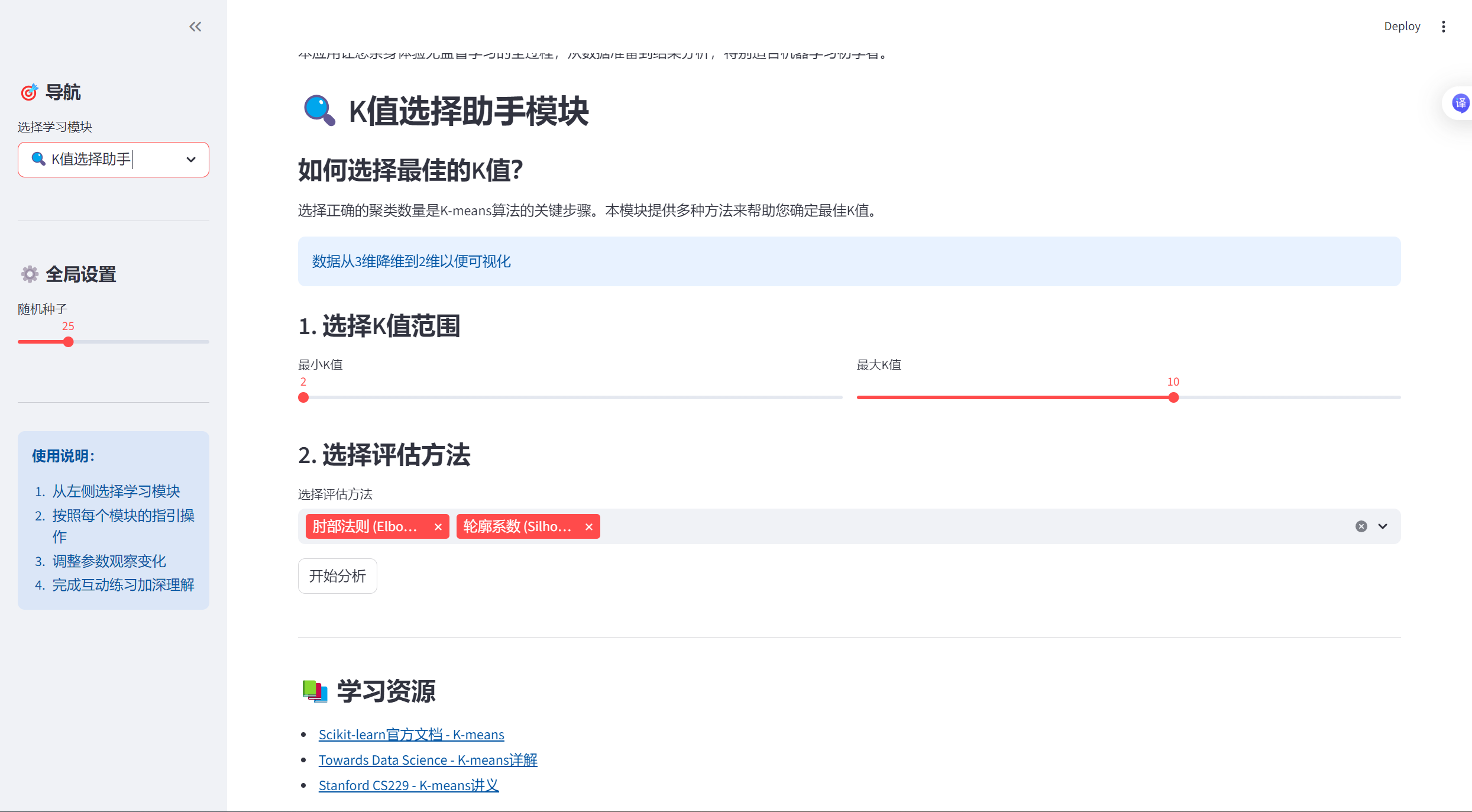
st.header("🔍 K值选择助手模块")
st.markdown("""
### 如何选择最佳的K值?
选择正确的聚类数量是K-means算法的关键步骤。本模块提供多种方法来帮助您确定最佳K值。
""")
# 检查是否有数据
if 'current_data' not in st.session_state or 'X' not in st.session_state.current_data:
st.warning("请先到'数据生成与探索'模块生成或上传数据。")
st.info("正在使用示例数据...")
X, _ = make_blobs(n_samples=300, centers=3, cluster_std=0.8, random_state=random_state)
else:
X = st.session_state.current_data['X']
# 如果数据维度高,使用PCA降维
if X.shape[1] > 2:
from sklearn.decomposition import PCA
pca = PCA(n_components=2)
X_vis = pca.fit_transform(X)
st.info(f"数据从{X.shape[1]}维降维到2维以便可视化")
else:
X_vis = X
# K值范围选择
st.subheader("1. 选择K值范围")
col1, col2 = st.columns(2)
with col1:
min_k = st.slider("最小K值", 2, 10, 2)
with col2:
max_k = st.slider("最大K值", min_k + 1, 15, 10)
k_range = range(min_k, max_k + 1)
# 计算方法选择
st.subheader("2. 选择评估方法")
method = st.multiselect(
"选择评估方法",
["肘部法则 (Elbow Method)", "轮廓系数 (Silhouette Score)", "簇间距离"],
default=["肘部法则 (Elbow Method)", "轮廓系数 (Silhouette Score)"]
)
if st.button("开始分析"):
# 计算不同K值下的指标
inertias = []
silhouette_scores = []
models = []
progress_bar = st.progress(0)
status_text = st.empty()
for i, k in enumerate(k_range):
status_text.text(f"计算 K={k}...")
# 训练K-means模型
kmeans = KMeans(n_clusters=k, random_state=random_state)
labels = kmeans.fit_predict(X_vis)
# 保存模型
models.append(kmeans)
# 计算惯量
inertias.append(kmeans.inertia_)
# 计算轮廓系数(需要至少2个簇)
if k > 1:
silhouette_scores.append(silhouette_score(X_vis, labels))
else:
silhouette_scores.append(0)
# 更新进度
progress_bar.progress((i + 1) / len(k_range))
status_text.text("分析完成!")
# 可视化结果
st.subheader("3. 分析结果")
# 创建多个图表
if "肘部法则 (Elbow Method)" in method:
# 肘部法则图
fig1, ax1 = plt.subplots(figsize=(10, 6))
ax1.plot(k_range, inertias, 'bo-', linewidth=2, markersize=8)
ax1.set_xlabel('聚类数量 (K)')
ax1.set_ylabel('惯量 (簇内平方和)')
ax1.set_title('肘部法则: 惯量随K值的变化')
ax1.grid(True, alpha=0.3)
# 标记可能的肘点
# 计算每个点的角度变化
if len(inertias) >= 3:
# 简单方法:找到下降速度明显变缓的点
differences = np.diff(inertias)
relative_differences = differences / inertias[:-1]
# 找到下降率变化最大的点
diff_of_diffs = np.diff(relative_differences)
if len(diff_of_diffs) > 0:
elbow_index = np.argmax(diff_of_diffs) + 1
if elbow_index < len(k_range):
elbow_k = list(k_range)[elbow_index]
ax1.axvline(x=elbow_k, color='r', linestyle='--', alpha=0.7)
ax1.text(elbow_k + 0.1, max(inertias) * 0.9,
f'建议K={elbow_k}', color='red', fontsize=12)
st.pyplot(fig1)
st.markdown("""
**肘部法则解释**:
- 惯量是每个数据点到其所属簇质心的距离平方和
- 随着K值增加,惯量会逐渐减小
- "肘部"是惯量下降速度明显变缓的点
- 这个点通常是最佳的K值选择
""")
if "轮廓系数 (Silhouette Score)" in method:
# 轮廓系数图
fig2, ax2 = plt.subplots(figsize=(10, 6))
ax2.plot(k_range, silhouette_scores, 'go-', linewidth=2, markersize=8)
ax2.set_xlabel('聚类数量 (K)')
ax2.set_ylabel('轮廓系数')
ax2.set_title('轮廓系数随K值的变化')
ax2.grid(True, alpha=0.3)
# 标记最大轮廓系数
if len(silhouette_scores) > 0:
max_index = np.argmax(silhouette_scores)
best_k = list(k_range)[max_index]
best_score = silhouette_scores[max_index]
ax2.axvline(x=best_k, color='r', linestyle='--', alpha=0.7)
ax2.plot(best_k, best_score, 'ro', markersize=12)
ax2.text(best_k + 0.1, best_score,
f'最佳K={best_k} (分数={best_score:.3f})',
color='red', fontsize=12)
st.pyplot(fig2)
st.markdown("""
**轮廓系数解释**:
- 轮廓系数衡量一个数据点与自身簇的相似度相对于其他簇的相似度
- 取值范围为[-1, 1],值越大表示聚类效果越好
- 值接近1:数据点被很好地分配到自己的簇
- 值接近0:数据点在两个簇的边界上
- 值接近-1:数据点可能被分配到了错误的簇
""")
# 综合推荐
st.subheader("4. 综合推荐")
col1, col2 = st.columns(2)
with col1:
if len(inertias) >= 3:
# 基于肘部法则的推荐
differences = np.diff(inertias)
relative_differences = differences / inertias[:-1]
diff_of_diffs = np.diff(relative_differences)
if len(diff_of_diffs) > 0:
elbow_index = np.argmax(diff_of_diffs) + 1
if elbow_index < len(k_range):
elbow_k = list(k_range)[elbow_index]
st.metric("肘部法则推荐K值", elbow_k)
with col2:
if len(silhouette_scores) > 0:
# 基于轮廓系数的推荐
max_index = np.argmax(silhouette_scores)
silhouette_k = list(k_range)[max_index]
st.metric("轮廓系数推荐K值", silhouette_k)
# 可视化不同K值的聚类结果
st.subheader("5. 不同K值聚类结果对比")
# 选择几个K值进行展示
if len(k_range) <= 5:
selected_ks = list(k_range)
else:
# 选择几个有代表性的K值
selected_ks = [min_k, min_k + 1,
min_k + (max_k - min_k) // 2,
max_k - 1, max_k]
selected_ks = list(set(selected_ks)) # 去重
selected_ks.sort()
# 创建子图
fig3, axes = plt.subplots(1, len(selected_ks), figsize=(5 * len(selected_ks), 5))
if len(selected_ks) == 1:
axes = [axes]
for idx, k in enumerate(selected_ks):
ax = axes[idx]
# 获取对应K值的模型
model_idx = list(k_range).index(k)
kmeans_model = models[model_idx]
labels = kmeans_model.predict(X_vis)
# 绘制聚类结果
colors = plt.cm.tab10(np.arange(k) / max(k, 1))
for cluster_id in range(k):
cluster_points = X_vis[labels == cluster_id]
if len(cluster_points) > 0:
ax.scatter(cluster_points[:, 0], cluster_points[:, 1],
color=colors[cluster_id], alpha=0.6,
edgecolors='black', linewidth=0.5)
# 绘制质心
ax.scatter(kmeans_model.cluster_centers_[:, 0],
kmeans_model.cluster_centers_[:, 1],
marker='*', s=200, c='red', edgecolors='black',
linewidth=1)
ax.set_title(f'K = {k}')
ax.set_xlabel('特征1' if X_vis.shape[1] == 2 else '主成分1')
if idx == 0:
ax.set_ylabel('特征2' if X_vis.shape[1] == 2 else '主成分2')
ax.grid(True, alpha=0.3)
plt.tight_layout()
st.pyplot(fig3)
# 保存最佳K值
st.session_state.current_data['best_k'] = selected_ks[2] if len(selected_ks) >= 3 else selected_ks[0]
# ==================== 实际应用场景模块 ====================
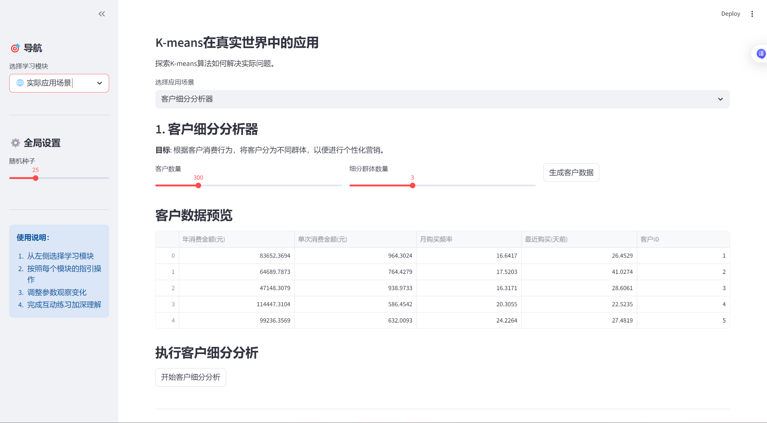
elif app_mode == "🌐 实际应用场景":
st.header("🌐 实际应用场景模块")
st.markdown("""
### K-means在真实世界中的应用
探索K-means算法如何解决实际问题。
""")
# 选择应用场景
scenario = st.selectbox(
"选择应用场景",
["客户细分分析器", "异常检测器", "图像颜色量化器"]
)
if scenario == "客户细分分析器":
st.subheader("1. 客户细分分析器")
st.markdown("""
**目标**: 根据客户消费行为,将客户分为不同群体,以便进行个性化营销。
""")
# 生成模拟客户数据
col1, col2, col3 = st.columns(3)
with col1:
n_customers = st.slider("客户数量", 100, 1000, 300)
with col2:
n_clusters = st.slider("细分群体数量", 2, 5, 3)
with col3:
generate_data = st.button("生成客户数据")
if generate_data or 'customer_data' not in st.session_state:
# 生成模拟客户数据
# 特征:年消费金额、单次消费金额、购买频率、最近购买时间
np.random.seed(random_state)
# 创建不同群体的客户
segments_centers = np.array([
[80000, 800, 20, 30], # VIP客户
[30000, 300, 8, 90], # 普通客户
[10000, 100, 2, 180], # 潜在流失客户
[50000, 500, 12, 60], # 高价值客户
[15000, 150, 4, 120] # 低价值客户
])[:n_clusters]
customer_data = []
for i, center in enumerate(segments_centers):
n_segment = n_customers // n_clusters
if i == n_clusters - 1:
n_segment = n_customers - (n_clusters - 1) * (n_customers // n_clusters)
# 为每个群体生成数据
segment_data = np.random.normal(loc=center, scale=center * 0.2, size=(n_segment, 4))
customer_data.append(segment_data)
customer_data = np.vstack(customer_data)
# 确保数据为正数
customer_data = np.abs(customer_data)
# 创建DataFrame
df_customers = pd.DataFrame(customer_data, columns=[
'年消费金额(元)', '单次消费金额(元)', '月购买频率', '最近购买(天前)'
])
# 添加客户ID
df_customers['客户ID'] = range(1, len(df_customers) + 1)
st.session_state.customer_data = df_customers
if 'customer_data' in st.session_state:
df_customers = st.session_state.customer_data
# 显示数据
st.subheader("客户数据预览")
st.dataframe(df_customers.head(), use_container_width=True)
# 执行聚类分析
st.subheader("执行客户细分分析")
if st.button("开始客户细分分析"):
# 选择用于聚类的特征
features = ['年消费金额(元)', '单次消费金额(元)', '月购买频率', '最近购买(天前)']
X = df_customers[features].values
# 标准化数据
scaler = StandardScaler()
X_scaled = scaler.fit_transform(X)
# 使用K-means聚类
kmeans = KMeans(n_clusters=n_clusters, random_state=random_state)
df_customers['客户群体'] = kmeans.fit_predict(X_scaled)
# 分析每个群体的特征
st.subheader("客户群体分析")
# 计算每个群体的平均特征值
segment_profiles = df_customers.groupby('客户群体')[features].mean().round(2)
# 添加群体描述
segment_descriptions = []
for i in range(n_clusters):
profile = segment_profiles.loc[i]
# 根据特征判断群体类型
if profile['年消费金额(元)'] > 60000 and profile['单次消费金额(元)'] > 600:
desc = "VIP客户"
elif profile['年消费金额(元)'] < 20000 and profile['最近购买(天前)'] > 150:
desc = "潜在流失客户"
elif profile['月购买频率'] > 15:
desc = "高活跃度客户"
elif profile['单次消费金额(元)'] > 500:
desc = "高价值客户"
else:
desc = "普通客户"
segment_descriptions.append(desc)
segment_profiles['群体描述'] = segment_descriptions
segment_profiles['客户数量'] = df_customers['客户群体'].value_counts().sort_index()
st.dataframe(segment_profiles, use_container_width=True)
# 可视化
st.subheader("客户群体可视化")
# 使用PCA降维到2D以便可视化
from sklearn.decomposition import PCA
pca = PCA(n_components=2)
X_pca = pca.fit_transform(X_scaled)
fig, ax = plt.subplots(figsize=(10, 7))
colors = plt.cm.Set3(np.arange(n_clusters) / max(n_clusters, 1))
for i in range(n_clusters):
cluster_points = X_pca[df_customers['客户群体'] == i]
ax.scatter(cluster_points[:, 0], cluster_points[:, 1],
color=colors[i], alpha=0.7, edgecolors='black',
linewidth=0.5, label=f'{segment_descriptions[i]} (群体{i})')
ax.set_xlabel('主成分1')
ax.set_ylabel('主成分2')
ax.set_title('客户细分结果')
ax.legend()
ax.grid(True, alpha=0.3)
st.pyplot(fig)
# 营销建议
st.subheader("个性化营销建议")
for i, desc in enumerate(segment_descriptions):
with st.expander(f"**{desc} (群体{i}) - {segment_profiles.loc[i, '客户数量']}名客户**"):
if desc == "VIP客户":
st.markdown("""
**营销策略**:
- 提供专属客服和优先服务
- 发放高价值礼品和专属折扣
- 邀请参加新品预览和专属活动
- 提供个性化产品推荐
**沟通频率**: 每周一次
**沟通渠道**: 电话、专属顾问、线下活动
""")
elif desc == "潜在流失客户":
st.markdown("""
**营销策略**:
- 发送再激活优惠券和特别折扣
- 了解流失原因并解决问题
- 提供个性化回归奖励
- 通过问卷调查了解需求变化
**沟通频率**: 每两周一次
**沟通渠道**: 邮件、短信、社交媒体
""")
elif desc == "高活跃度客户":
st.markdown("""
**营销策略**:
- 提供忠诚度计划和积分奖励
- 推荐相关产品或套餐
- 邀请参与产品反馈和测试
- 提供专属社区或论坛访问
**沟通频率**: 每周一次
**沟通渠道**: App推送、邮件、社交媒体
""")
elif desc == "高价值客户":
st.markdown("""
**营销策略**:
- 提供升级套餐或高级服务
- 推荐高价值产品或服务
- 提供专属折扣和促销活动
- 邀请参与高端客户活动
**沟通频率**: 每两周一次
**沟通渠道**: 邮件、电话、专属顾问
""")
else: # 普通客户
st.markdown("""
**营销策略**:
- 提供基础忠诚度计划
- 定期发送促销信息和优惠券
- 推荐热门产品或服务
- 通过内容营销增加互动
**沟通频率**: 每月一次
**沟通渠道**: 邮件、社交媒体、App推送
""")
elif scenario == "异常检测器":
st.subheader("2. 异常检测器")
st.markdown("""
**目标**: 识别学生行为数据中的异常模式,如可能作弊的学生。
""")
# 生成模拟学生数据
col1, col2 = st.columns(2)
with col1:
n_students = st.slider("学生数量", 50, 500, 100)
with col2:
anomaly_percent = st.slider("异常学生比例 (%)", 1, 20, 5)
if st.button("生成学生数据"):
# 生成正常学生数据
np.random.seed(random_state)
# 正常学生:学习时间和成绩正相关
n_normal = int(n_students * (1 - anomaly_percent / 100))
# 基础学习时间
study_hours = np.random.normal(20, 5, n_normal)
study_hours = np.clip(study_hours, 5, 40)
# 成绩与学习时间相关,但有随机性
scores = 50 + study_hours * 1.5 + np.random.normal(0, 8, n_normal)
scores = np.clip(scores, 0, 100)
normal_data = np.column_stack([study_hours, scores])
normal_labels = ['正常'] * n_normal
# 生成异常学生数据
n_anomaly = n_students - n_normal
# 类型1: 学习时间少但成绩高(可能作弊)
anomaly1_hours = np.random.uniform(5, 15, n_anomaly // 2)
anomaly1_scores = np.random.uniform(85, 100, n_anomaly // 2)
anomaly1_data = np.column_stack([anomaly1_hours, anomaly1_scores])
anomaly1_labels = ['可能作弊'] * (n_anomaly // 2)
# 类型2: 学习时间多但成绩低(可能需要帮助)
anomaly2_hours = np.random.uniform(30, 40, n_anomaly - n_anomaly // 2)
anomaly2_scores = np.random.uniform(40, 60, n_anomaly - n_anomaly // 2)
anomaly2_data = np.column_stack([anomaly2_hours, anomaly2_scores])
anomaly2_labels = ['需要帮助'] * (n_anomaly - n_anomaly // 2)
# 合并所有数据
all_data = np.vstack([normal_data, anomaly1_data, anomaly2_data])
all_labels = normal_labels + anomaly1_labels + anomaly2_labels
# 创建DataFrame
df_students = pd.DataFrame(all_data, columns=['学习时间(小时/周)', '考试成绩(分)'])
df_students['真实状态'] = all_labels
df_students['学生ID'] = range(1, len(df_students) + 1)
# 打乱数据
df_students = df_students.sample(frac=1, random_state=random_state).reset_index(drop=True)
st.session_state.student_data = df_students
if 'student_data' in st.session_state:
df_students = st.session_state.student_data
# 显示数据
st.subheader("学生数据预览")
st.dataframe(df_students.head(), use_container_width=True)
# 可视化原始数据
fig, ax = plt.subplots(figsize=(10, 6))
# 根据真实状态着色
colors = {'正常': 'blue', '可能作弊': 'red', '需要帮助': 'orange'}
for status in df_students['真实状态'].unique():
subset = df_students[df_students['真实状态'] == status]
ax.scatter(subset['学习时间(小时/周)'], subset['考试成绩(分)'],
color=colors.get(status, 'gray'), alpha=0.7,
edgecolors='black', linewidth=0.5, label=status)
ax.set_xlabel('学习时间(小时/周)')
ax.set_ylabel('考试成绩(分)')
ax.set_title('学生行为数据分布')
ax.legend()
ax.grid(True, alpha=0.3)
st.pyplot(fig)
# 执行异常检测
st.subheader("执行异常检测")
if st.button("开始异常检测"):
# 准备数据
X = df_students[['学习时间(小时/周)', '考试成绩(分)']].values
# 标准化数据
scaler = StandardScaler()
X_scaled = scaler.fit_transform(X)
# 使用K-means进行异常检测
# 使用较小的K值,将数据分为几个主要群体
kmeans = KMeans(n_clusters=3, random_state=random_state)
cluster_labels = kmeans.fit_predict(X_scaled)
# 计算每个点到其质心的距离
distances = np.sqrt(((X_scaled - kmeans.cluster_centers_[cluster_labels]) ** 2).sum(axis=1))
# 根据距离判断异常
threshold = np.percentile(distances, 90) # 距离最大的10%被认为是异常
df_students['异常得分'] = distances
df_students['检测结果'] = np.where(distances > threshold, '异常', '正常')
# 显示结果
st.subheader("异常检测结果")
# 创建混淆矩阵
from sklearn.metrics import confusion_matrix, classification_report
# 简化真实标签:将"正常"视为正常,其他视为异常
true_labels = df_students['真实状态'].apply(lambda x: '正常' if x == '正常' else '异常')
pred_labels = df_students['检测结果']
# 计算混淆矩阵
cm = confusion_matrix(true_labels, pred_labels, labels=['正常', '异常'])
# 显示混淆矩阵
fig, ax = plt.subplots(figsize=(6, 5))
im = ax.imshow(cm, interpolation='nearest', cmap=plt.cm.Blues)
ax.figure.colorbar(im, ax=ax)
# 添加标签
classes = ['正常', '异常']
ax.set(xticks=np.arange(cm.shape[1]),
yticks=np.arange(cm.shape[0]),
xticklabels=classes, yticklabels=classes,
title='混淆矩阵',
ylabel='真实标签',
xlabel='预测标签')
# 在格子中添加数字
thresh = cm.max() / 2.
for i in range(cm.shape[0]):
for j in range(cm.shape[1]):
ax.text(j, i, format(cm[i, j], 'd'),
ha="center", va="center",
color="white" if cm[i, j] > thresh else "black")
plt.tight_layout()
st.pyplot(fig)
# 显示分类报告
st.subheader("分类报告")
report = classification_report(true_labels, pred_labels, output_dict=True)
report_df = pd.DataFrame(report).transpose()
st.dataframe(report_df, use_container_width=True)
# 可视化异常检测结果
fig, (ax1, ax2) = plt.subplots(1, 2, figsize=(15, 6))
# 图1: 真实状态
for status in df_students['真实状态'].unique():
subset = df_students[df_students['真实状态'] == status]
ax1.scatter(subset['学习时间(小时/周)'], subset['考试成绩(分)'],
color=colors.get(status, 'gray'), alpha=0.7,
edgecolors='black', linewidth=0.5, label=status)
ax1.set_xlabel('学习时间(小时/周)')
ax1.set_ylabel('考试成绩(分)')
ax1.set_title('真实学生状态')
ax1.legend()
ax1.grid(True, alpha=0.3)
# 图2: 检测结果
detect_colors = {'正常': 'green', '异常': 'red'}
for result in df_students['检测结果'].unique():
subset = df_students[df_students['检测结果'] == result]
ax2.scatter(subset['学习时间(小时/周)'], subset['考试成绩(分)'],
color=detect_colors.get(result, 'gray'), alpha=0.7,
edgecolors='black', linewidth=0.5, label=result)
ax2.set_xlabel('学习时间(小时/周)')
ax2.set_ylabel('考试成绩(分)')
ax2.set_title('异常检测结果')
ax2.legend()
ax2.grid(True, alpha=0.3)
plt.tight_layout()
st.pyplot(fig)
# 显示异常学生详细信息
st.subheader("检测到的异常学生")
anomaly_students = df_students[df_students['检测结果'] == '异常']
st.dataframe(anomaly_students[
['学生ID', '学习时间(小时/周)', '考试成绩(分)', '真实状态', '异常得分']].sort_values(
'异常得分', ascending=False),
use_container_width=True)
# 异常原因分析
st.subheader("异常原因分析")
for idx, row in anomaly_students.iterrows():
with st.expander(
f"学生 {int(row['学生ID'])}: 学习时间={row['学习时间(小时/周)']:.1f}小时, 成绩={row['考试成绩(分)']:.1f}分"):
if row['学习时间(小时/周)'] < 15 and row['考试成绩(分)'] > 85:
st.markdown(f"""
**可能原因**: 学习时间较少但成绩很高
**风险等级**: 高
**建议行动**:
1. 检查是否存在作弊行为
2. 进行额外的口头测试
3. 了解学生的学习方法
4. 与家长沟通情况
""")
elif row['学习时间(小时/周)'] > 30 and row['考试成绩(分)'] < 60:
st.markdown(f"""
**可能原因**: 学习时间很长但成绩较低
**风险等级**: 中
**建议行动**:
1. 评估学习方法是否有效
2. 提供学习技巧指导
3. 检查是否存在学习障碍
4. 考虑额外的辅导支持
""")
else:
st.markdown(f"""
**可能原因**: 行为模式与大多数学生不同
**风险等级**: 低
**建议行动**:
1. 进一步观察学生表现
2. 与学生进行一对一交流
3. 收集更多行为数据
""")
elif scenario == "图像颜色量化器":
st.subheader("3. 图像颜色量化器")
st.markdown("""
**目标**: 使用K-means减少图像中的颜色数量,实现图像压缩。
""")
# 图像上传
uploaded_image = st.file_uploader("上传图像文件", type=['jpg', 'jpeg', 'png'])
if uploaded_image is not None:
# 读取图像
image = Image.open(uploaded_image)
# 显示原始图像
st.subheader("原始图像")
st.image(image, caption=f"原始图像 - 大小: {image.size}", use_column_width=True)
# 颜色数量设置
col1, col2 = st.columns(2)
with col1:
n_colors = st.slider("目标颜色数量", 2, 64, 16)
with col2:
process_image = st.button("处理图像")
if process_image:
# 将图像转换为numpy数组
img_array = np.array(image)
# 获取图像尺寸
height, width = img_array.shape[:2]
# 将图像重塑为2D数组 (像素 x RGB)
if len(img_array.shape) == 3:
# 彩色图像
img_reshaped = img_array.reshape(-1, 3)
else:
# 灰度图像
img_reshaped = img_array.reshape(-1, 1)
# 使用K-means进行颜色量化
st.info(f"正在使用K-means将颜色从数千种减少到{n_colors}种...")
kmeans = KMeans(n_clusters=n_colors, random_state=random_state)
labels = kmeans.fit_predict(img_reshaped)
# 用质心颜色替换每个像素的颜色
quantized_colors = kmeans.cluster_centers_.astype(int)
quantized_img = quantized_colors[labels].reshape(img_array.shape)
# 显示量化后的图像
st.subheader("颜色量化后的图像")
quantized_image = Image.fromarray(quantized_img.astype('uint8'))
st.image(quantized_image, caption=f"量化后图像 - 颜色数量: {n_colors}", use_column_width=True)
# 显示颜色调色板
st.subheader("颜色调色板")
# 创建颜色调色板可视化
fig, ax = plt.subplots(figsize=(10, 2))
# 显示颜色块
for i, color in enumerate(quantized_colors):
if len(color) == 3:
color = color / 255.0 # 归一化到[0, 1]
rect = plt.Rectangle((i, 0), 1, 1, color=color)
else:
# 灰度图像
gray = color[0] / 255.0
rect = plt.Rectangle((i, 0), 1, 1, color=(gray, gray, gray))
ax.add_patch(rect)
ax.set_xlim(0, len(quantized_colors))
ax.set_ylim(0, 1)
ax.set_aspect('equal')
ax.axis('off')
ax.set_title(f'量化后的{len(quantized_colors)}种颜色')
st.pyplot(fig)
# 计算压缩比
if len(img_array.shape) == 3:
original_size = height * width * 3 # 每个像素3个通道
# 量化后:每个像素存储簇索引(需要log2(n_colors)位) + 颜色调色板
compressed_size = height * width * np.ceil(np.log2(n_colors)) / 8 + n_colors * 3
compression_ratio = original_size / compressed_size
else:
original_size = height * width
compressed_size = height * width * np.ceil(np.log2(n_colors)) / 8 + n_colors
compression_ratio = original_size / compressed_size
# 显示统计信息
col1, col2, col3 = st.columns(3)
with col1:
st.metric("原始图像尺寸", f"{height} × {width}")
with col2:
if len(img_array.shape) == 3:
st.metric("颜色数量", f"数千 → {n_colors}")
else:
st.metric("灰度级别", f"256 → {n_colors}")
with col3:
st.metric("压缩比", f"{compression_ratio:.1f}:1")
# 并排显示对比
st.subheader("对比图")
fig, (ax1, ax2) = plt.subplots(1, 2, figsize=(12, 6))
ax1.imshow(image)
ax1.set_title('原始图像')
ax1.axis('off')
ax2.imshow(quantized_image)
ax2.set_title(f'量化后图像 ({n_colors}种颜色)')
ax2.axis('off')
plt.tight_layout()
st.pyplot(fig)
# 提供下载链接
st.subheader("下载处理后的图像")
# 将图像转换为字节
from io import BytesIO
buffered = BytesIO()
quantized_image.save(buffered, format="PNG")
img_str = base64.b64encode(buffered.getvalue()).decode()
href = f'<a href="data:file/png;base64,{img_str}" download="quantized_image.png">点击下载量化后的图像</a>'
st.markdown(href, unsafe_allow_html=True)
else:
# 提供示例图像
st.info("请上传图像文件,或使用以下示例图像")
# 创建示例图像
example_option = st.selectbox("选择示例图像", ["渐变图像", "简单图形", "测试图案"])
if example_option == "渐变图像":
# 创建渐变图像
gradient = np.zeros((200, 300, 3), dtype=np.uint8)
for i in range(300):
gradient[:, i, 0] = int(255 * i / 300) # 红色通道渐变
gradient[:, i, 1] = int(255 * (1 - i / 300)) # 绿色通道渐变
gradient[:, i, 2] = 128 # 固定蓝色通道
image = Image.fromarray(gradient)
st.image(image, caption="示例渐变图像", use_column_width=True)
# 保存到session state以便后续处理
st.session_state.example_image = gradient
elif example_option == "简单图形":
# 创建简单图形
img = np.zeros((200, 300, 3), dtype=np.uint8)
# 红色矩形
img[50:100, 50:100, 0] = 255
# 绿色圆形
for i in range(200):
for j in range(300):
if (i - 150) ** 2 + (j - 100) ** 2 < 400: # 半径20
img[i, j, 1] = 255
# 蓝色三角形
for i in range(200):
for j in range(300):
if i > 100 and j > 200 and (i - 100) < (j - 200):
img[i, j, 2] = 255
image = Image.fromarray(img)
st.image(image, caption="示例简单图形", use_column_width=True)
st.session_state.example_image = img
else: # 测试图案
# 创建测试图案
img = np.zeros((200, 300, 3), dtype=np.uint8)
# 棋盘格
for i in range(200):
for j in range(300):
if (i // 20 + j // 20) % 2 == 0:
img[i, j, :] = [255, 255, 255] # 白色
else:
img[i, j, :] = [0, 0, 0] # 黑色
image = Image.fromarray(img)
st.image(image, caption="示例测试图案", use_column_width=True)
st.session_state.example_image = img
# ==================== 交互式学习模块 ====================
elif app_mode == "🎓 交互式学习":
st.header("🎓 交互式学习模块")
st.markdown("""
### 通过互动练习巩固K-means知识
在这个模块中,您可以通过各种互动练习来加深对K-means算法的理解。
""")
# 选择学习活动
activity = st.selectbox(
"选择学习活动",
["概念选择题", "拖动练习题", "预测游戏", "算法优缺点对比"]
)
if activity == "概念选择题":
st.subheader("概念选择题")
st.markdown("测试您对K-means算法的理解。")
# 问题1
st.markdown("### 问题 1: 什么是质心(centroid)?")
answer1 = st.radio(
"选择正确答案:",
["A. 数据集中最中间的点",
"B. 一个簇中所有数据点的平均值",
"C. 离所有点最近的数据点",
"D. 数据集中最大值和最小值的中间点"],
key="q1"
)
if st.button("检查答案1"):
if answer1 == "B. 一个簇中所有数据点的平均值":
st.success("✅ 正确!质心是一个簇中所有数据点的平均值(均值点)。")
else:
st.error("❌ 不正确。质心是一个簇中所有数据点的平均值。")
st.markdown("---")
# 问题2
st.markdown("### 问题 2: K-means算法的目标是什么?")
answer2 = st.radio(
"选择正确答案:",
["A. 最大化簇间距离",
"B. 最小化簇内平方和(惯量)",
"C. 最大化数据点到质心的总距离",
"D. 最小化数据点的数量"],
key="q2"
)
if st.button("检查答案2"):
if answer2 == "B. 最小化簇内平方和(惯量)":
st.success("✅ 正确!K-means的目标是最小化簇内平方和,即使每个数据点尽可能接近其所属簇的质心。")
else:
st.error("❌ 不正确。K-means的目标是最小化簇内平方和(惯量)。")
st.markdown("---")
# 问题3
st.markdown("### 问题 3: 如何选择最佳的K值?")
answer3 = st.multiselect(
"选择所有适用的方法:",
["A. 随机选择一个K值",
"B. 使用肘部法则(Elbow Method)",
"C. 使用轮廓系数(Silhouette Score)",
"D. 总是选择K=3",
"E. 根据业务需求或领域知识"],
key="q3"
)
if st.button("检查答案3"):
correct_answers = ["B. 使用肘部法则(Elbow Method)",
"C. 使用轮廓系数(Silhouette Score)",
"E. 根据业务需求或领域知识"]
if set(answer3) == set(correct_answers):
st.success("✅ 完全正确!这三种都是选择K值的有效方法。")
elif any(item in correct_answers for item in answer3):
st.warning("⚠️ 部分正确。正确的方法是:肘部法则、轮廓系数和根据业务需求选择。")
else:
st.error("❌ 不正确。正确的方法是:肘部法则、轮廓系数和根据业务需求选择。")
st.markdown("---")
# 问题4
st.markdown("### 问题 4: K-means算法的局限性是什么?")
answer4 = st.multiselect(
"选择所有适用的选项:",
["A. 需要预先指定K值",
"B. 对初始质心位置敏感",
"C. 只能处理数值数据",
"D. 假设簇是球形的且大小相似",
"E. 对异常值敏感"],
key="q4"
)
if st.button("检查答案4"):
correct_answers = ["A. 需要预先指定K值",
"B. 对初始质心位置敏感",
"D. 假设簇是球形的且大小相似",
"E. 对异常值敏感"]
if set(answer4) == set(correct_answers):
st.success("✅ 完全正确!这些都是K-means的局限性。")
elif any(item in correct_answers for item in answer4):
st.warning(
"⚠️ 部分正确。K-means的主要局限性包括:需要预先指定K值、对初始质心敏感、假设球形簇、对异常值敏感。")
else:
st.error("❌ 不正确。K-means的主要局限性包括:需要预先指定K值、对初始质心敏感、假设球形簇、对异常值敏感。")
# 显示分数
st.markdown("---")
if st.button("计算总分"):
score = 0
total = 4
if answer1 == "B. 一个簇中所有数据点的平均值":
score += 1
if answer2 == "B. 最小化簇内平方和(惯量)":
score += 1
correct_q3 = ["B. 使用肘部法则(Elbow Method)",
"C. 使用轮廓系数(Silhouette Score)",
"E. 根据业务需求或领域知识"]
if set(answer3) == set(correct_q3):
score += 1
correct_q4 = ["A. 需要预先指定K值",
"B. 对初始质心位置敏感",
"D. 假设簇是球形的且大小相似",
"E. 对异常值敏感"]
if set(answer4) == set(correct_q4):
score += 1
st.success(f"您的得分: {score}/{total}")
if score == total:
st.balloons()
elif activity == "拖动练习题":
st.subheader("拖动练习题")
st.markdown("""
### 手动调整质心位置
在这个练习中,您可以手动拖动质心,观察K-means算法如何重新分配数据点。
""")
# 生成简单的数据
np.random.seed(random_state)
X = np.random.randn(50, 2) * 0.5
X[:25, 0] += 2
X[25:, 0] -= 2
# 创建初始质心位置
initial_centroids = np.array([[-2, 0], [2, 0]])
# 使用plotly创建交互式图表
fig = go.Figure()
# 添加数据点
fig.add_trace(go.Scatter(
x=X[:, 0],
y=X[:, 1],
mode='markers',
marker=dict(size=10, color='lightblue', line=dict(width=1, color='black')),
name='数据点',
hoverinfo='text',
text=[f'点 {i + 1}' for i in range(len(X))]
))
# 添加初始质心
fig.add_trace(go.Scatter(
x=initial_centroids[:, 0],
y=initial_centroids[:, 1],
mode='markers',
marker=dict(size=20, symbol='star', color='red', line=dict(width=2, color='black')),
name='质心',
hoverinfo='text',
text=['质心 1', '质心 2']
))
# 更新布局
fig.update_layout(
title="拖动质心位置",
xaxis_title="X轴",
yaxis_title="Y轴",
hovermode='closest',
width=800,
height=600,
dragmode='pan' # 允许拖动
)
# 显示图表
st.plotly_chart(fig, use_container_width=True)
# 解释说明
st.markdown("""
**练习说明**:
1. 尝试拖动红色星形质心到不同位置
2. 观察数据点如何根据最近质心重新分配
3. 思考质心位置如何影响聚类结果
**提示**:
- 将质心拖动到数据密集的区域
- 尝试将两个质心放在同一区域,观察会发生什么
- 将质心放在远离所有数据点的位置
""")
# 添加重置按钮
if st.button("重置质心位置"):
st.rerun()
elif activity == "预测游戏":
st.subheader("预测游戏")
st.markdown("""
### 预测新数据点的簇标签
在这个游戏中,您需要预测新数据点属于哪个簇。
""")
# 生成聚类数据
np.random.seed(random_state)
n_clusters = 3
X, true_labels = make_blobs(n_samples=100, centers=n_clusters, cluster_std=0.8, random_state=random_state)
# 训练K-means模型
kmeans = KMeans(n_clusters=n_clusters, random_state=random_state)
kmeans.fit(X)
# 显示现有聚类
fig, ax = plt.subplots(figsize=(8, 6))
colors = plt.cm.tab10(np.arange(n_clusters) / max(n_clusters, 1))
for i in range(n_clusters):
cluster_points = X[kmeans.labels_ == i]
ax.scatter(cluster_points[:, 0], cluster_points[:, 1],
color=colors[i], alpha=0.7, edgecolors='black',
linewidth=0.5, label=f'簇 {i + 1}')
# 绘制质心
ax.scatter(kmeans.cluster_centers_[:, 0], kmeans.cluster_centers_[:, 1],
marker='*', s=200, c='red', edgecolors='black',
linewidth=1, label='质心')
ax.set_xlabel('特征1')
ax.set_ylabel('特征2')
ax.set_title('现有聚类')
ax.legend()
ax.grid(True, alpha=0.3)
st.pyplot(fig)
# 生成新数据点
st.markdown("### 新数据点")
col1, col2 = st.columns(2)
with col1:
new_x = st.slider("新点的X坐标", float(X[:, 0].min()), float(X[:, 0].max()), 0.0)
with col2:
new_y = st.slider("新点的Y坐标", float(X[:, 1].min()), float(X[:, 1].max()), 0.0)
new_point = np.array([[new_x, new_y]])
# 让用户预测
st.markdown("### 您的预测")
prediction = st.radio(
"您认为新数据点属于哪个簇?",
[f"簇 {i + 1}" for i in range(n_clusters)],
index=0
)
if st.button("提交预测"):
# 计算真实预测
true_pred = kmeans.predict(new_point)[0]
user_pred = int(prediction.split()[-1]) - 1 # 提取簇编号
# 显示结果
fig2, ax2 = plt.subplots(figsize=(8, 6))
# 绘制现有聚类
for i in range(n_clusters):
cluster_points = X[kmeans.labels_ == i]
ax2.scatter(cluster_points[:, 0], cluster_points[:, 1],
color=colors[i], alpha=0.7, edgecolors='black',
linewidth=0.5, label=f'簇 {i + 1}')
# 绘制质心
ax2.scatter(kmeans.cluster_centers_[:, 0], kmeans.cluster_centers_[:, 1],
marker='*', s=200, c='red', edgecolors='black',
linewidth=1, label='质心')
# 绘制新数据点
if user_pred == true_pred:
point_color = 'green'
result_text = "✅ 正确!"
else:
point_color = 'orange'
result_text = f"❌ 不正确。正确结果是:簇 {true_pred + 1}"
ax2.scatter(new_x, new_y, s=150, c=point_color,
edgecolors='black', linewidth=2, marker='D',
label='新数据点')
# 绘制到每个质心的距离
for i, center in enumerate(kmeans.cluster_centers_):
distance = np.sqrt((new_x - center[0]) ** 2 + (new_y - center[1]) ** 2)
ax2.plot([new_x, center[0]], [new_y, center[1]],
'gray', linestyle='--', alpha=0.5)
ax2.text((new_x + center[0]) / 2, (new_y + center[1]) / 2,
f'{distance:.2f}', fontsize=9,
bbox=dict(boxstyle="round,pad=0.3", facecolor="white", alpha=0.7))
ax2.set_xlabel('特征1')
ax2.set_ylabel('特征2')
ax2.set_title(f'预测结果: {result_text}')
ax2.legend()
ax2.grid(True, alpha=0.3)
st.pyplot(fig2)
# 显示解释
st.markdown("### 解释")
# 计算到每个质心的距离
distances = []
for i, center in enumerate(kmeans.cluster_centers_):
distance = np.sqrt((new_x - center[0]) ** 2 + (new_y - center[1]) ** 2)
distances.append((i, distance))
# 按距离排序
distances.sort(key=lambda x: x[1])
st.markdown(f"**距离计算**:")
for i, dist in distances:
st.markdown(f"- 到簇 {i + 1} 质心的距离: **{dist:.3f}**")
st.markdown(f"**K-means决策**: 将新点分配到最近的簇,即**簇 {distances[0][0] + 1}**")
if user_pred == true_pred:
st.success("恭喜!您的预测是正确的!")
else:
st.info(f"提示:K-means根据最近质心分配数据点。新点离簇 {distances[0][0] + 1} 的质心最近。")
# 添加新游戏按钮
if st.button("新游戏"):
st.rerun()
else: # 算法优缺点对比
st.subheader("算法优缺点对比")
st.markdown("""
### K-means与其他聚类算法的比较
了解K-means的优势和局限性,以及何时使用它。
""")
# 创建对比表格
algorithms = {
"K-means": {
"优点": [
"简单、直观、易于实现",
"对于球形簇效果很好",
"计算效率高,适合大数据集",
"可扩展性好"
],
"缺点": [
"需要预先指定K值",
"对初始质心敏感",
"对异常值敏感",
"假设簇是球形的且大小相似",
"可能收敛到局部最优"
],
"适用场景": [
"客户细分",
"图像压缩",
"文档聚类",
"异常检测"
]
},
"层次聚类": {
"优点": [
"不需要预先指定簇数",
"可以生成树状图(dendrogram)",
"可以发现任意形状的簇"
],
"缺点": [
"计算复杂度高(O(n³))",
"对噪声和异常值敏感",
"结果不可逆"
],
"适用场景": [
"小规模数据集",
"需要层次结构的场景",
"生物学分类"
]
},
"DBSCAN": {
"优点": [
"不需要预先指定簇数",
"可以发现任意形状的簇",
"对噪声鲁棒",
"可以识别异常点"
],
"缺点": [
"对参数(ε, minPts)敏感",
"不适用于密度差异大的数据集",
"高维数据效果差"
],
"适用场景": [
"空间数据聚类",
"异常检测",
"形状不规则的簇"
]
},
"高斯混合模型(GMM)": {
"优点": [
"提供概率聚类",
"可以处理不同大小的簇",
"可以处理相关性"
],
"缺点": [
"可能收敛到局部最优",
"需要指定簇数",
"计算复杂度较高"
],
"适用场景": [
"语音识别",
"图像分割",
"需要概率输出的场景"
]
}
}
# 显示对比表格
st.markdown("### 算法对比表")
# 选择要对比的算法
selected_algorithms = st.multiselect(
"选择要对比的算法:",
list(algorithms.keys()),
default=["K-means", "层次聚类", "DBSCAN"]
)
if selected_algorithms:
# 创建对比表格
for algo in selected_algorithms:
with st.expander(f"**{algo}**", expanded=True):
col1, col2, col3 = st.columns(3)
with col1:
st.markdown("**优点**")
for advantage in algorithms[algo]["优点"]:
st.markdown(f"- {advantage}")
with col2:
st.markdown("**缺点**")
for disadvantage in algorithms[algo]["缺点"]:
st.markdown(f"- {disadvantage}")
with col3:
st.markdown("**适用场景**")
for scenario in algorithms[algo]["适用场景"]:
st.markdown(f"- {scenario}")
# K-means最佳实践
st.markdown("---")
st.subheader("K-means最佳实践")
col1, col2 = st.columns(2)
with col1:
st.markdown("""
**什么时候使用K-means?**
- 数据集较大,需要高效算法
- 簇大致是球形的
- 簇的大小和密度相似
- 需要简单、可解释的结果
- 可以合理估计K值
**示例应用**:
- 客户细分
- 市场篮分析
- 图像颜色量化
- 文档主题建模
""")
with col2:
st.markdown("""
**如何改进K-means?**
- 使用K-means++初始化
- 多次运行选择最佳结果
- 使用肘部法则或轮廓系数选择K
- 预处理数据:标准化、去噪
- 结合领域知识解释结果
**常见陷阱**:
- 假设K值已知
- 忽略异常值的影响
- 未标准化不同尺度的特征
- 未验证聚类结果的有效性
""")
# 交互式练习:选择算法
st.markdown("---")
st.subheader("练习:为场景选择算法")
scenario = st.selectbox(
"选择场景:",
["1. 电商网站需要将100万客户分为5个群体进行精准营销",
"2. 生物学家需要根据基因表达数据对细胞进行分类,不知道类别数量",
"3. 城市规划师需要根据人口密度和设施分布划分城市区域",
"4. 银行需要检测信用卡交易中的异常模式"]
)
algorithm_choice = st.selectbox(
"您会选择哪种算法?",
["K-means", "层次聚类", "DBSCAN", "高斯混合模型(GMM)"],
key="scenario_choice"
)
if st.button("检查选择"):
if scenario.startswith("1.") and algorithm_choice == "K-means":
st.success("✅ 正确选择!K-means适合大数据集的客户细分,且电商通常能合理估计客户群体数量。")
elif scenario.startswith("2.") and algorithm_choice == "层次聚类":
st.success(
"✅ 正确选择!层次聚类适合不知道类别数量的场景,且可以生成树状图帮助生物学家理解细胞间的层次关系。")
elif scenario.startswith("3.") and algorithm_choice == "DBSCAN":
st.success("✅ 正确选择!DBSCAN适合空间数据聚类,可以发现任意形状的区域,且对噪声鲁棒。")
elif scenario.startswith("4.") and algorithm_choice in ["DBSCAN", "K-means"]:
st.success("✅ 合理选择!两者都可用于异常检测:DBSCAN直接识别异常点,K-means通过距离质心的距离检测异常。")
else:
st.info(
"💡 思考:考虑数据特点、问题需求和算法特性。场景1适合K-means,场景2适合层次聚类,场景3适合DBSCAN,场景4适合DBSCAN或K-means。")
# 页脚
st.markdown("---")
st.markdown("""
### 📚 学习资源
- [Scikit-learn官方文档 - K-means](https://scikit-learn.org/stable/modules/clustering.html#k-means)
- [Towards Data Science - K-means详解](https://towardsdatascience.com/k-means-clustering-algorithm-applications-evaluation-methods-and-drawbacks-aa03e644b48a)
- [Stanford CS229 - K-means讲义](http://cs229.stanford.edu/notes/cs229-notes7a.pdf)
### 💡 提示
- 尝试调整不同参数观察效果变化
- 在实际数据集上练习K-means应用
- 理解算法的局限性,知道何时不使用K-means
""")
st.caption("© 2025 K-means智能客户分群与可视化分析系统 | 为机器学习初学者设计 | free-elcmacom")