在人工智能的众多分支中,自然语言处理(NLP)一直是最具挑战性的领域之一。要让机器理解、生成人类语言,核心在于解决两个基本问题:
- 如何用数字表示文本?(文本表示问题)
- 如何计算文本的概率?(语言模型问题)
| 技术名称 | 技术类型 | 训练目标 | 核心输出 | 典型应用 | 出现时间 | 技术特点 |
|---|---|---|---|---|---|---|
| One-Hot | 文本表示 | 无 | 稀疏二值向量 | 分类变量编码 | 早期 | 离散、稀疏、高维、无语义 |
| 词袋模型 | 文本表示 | 无 | 词频向量 | 文档分类、信息检索 | 早期 | 忽略顺序、统计词频、无语义 |
| TF-IDF | 文本表示 | 加权统计 | 加权词频向量 | 信息检索、文本分类 | 1972 | 权重优化、突出关键词、无语义 |
| N-gram | 语言模型 | 统计词序列概率 | 概率分布 | 文本补全、语音识别 | 1990s | 马尔可夫假设、局部依赖、统计基础 |
| NNLM前馈神经网络语言模型 | 语言模型 | 分布式表示 | 预测下一个词 | 泛化能力更强 | 2003 | 前馈神经网络、词嵌入 |
| RNN/LSTM语言模型 | 语言模型 | 循环连接 | 序列生成概率 | 长序列建模 | 2010 | 循环神经网络、记忆机制 |
| Transformer语言模型 | 自注意力模型 | 注意力机制 | 并行序列生成 | 长程依赖捕捉 | 2017 | 自注意力、并行计算 |
| Word2Vec | 文本表示为主,语言模型为次 | 预测上下文词 | 静态词向量 | 词相似度、词类比 | 2013 | 分布式表示、语义相似、静态向量 |
| GloVe | 文本表示 | 矩阵分解 | 静态词向量 | 词相似度、初始表示 | 2014 | 全局+局部、共现矩阵、静态向量 |
| ELMo | 文本表示为主,语言模型为次 | 双向语言模型 | 上下文词向量 | 特征提取、一词多义 | 2018 | 双向LSTM、多层融合、动态表示 |
| BERT | 文本表示为主,语言模型为次 | 掩码语言模型 | 上下文表示 | 文本分类、问答系统 | 2018 | 双向Transformer、MLM、动态表示 |
| GPT系列 | 语言模型为主,文本表示为次 | 自回归生成 | 生成概率+向量 | 文本生成、对话系统 | 2018- | 自回归、生成能力强、单向上下文 |
一、离散表示时代
1.1 One-Hot 编码
One-Hot编码是分类变量最基本的表示方法。其核心思想是为每个类别创建一个二进制向量,向量的长度等于类别总数,其中只有对应类别的位置为1,其余为0。例如,词汇表["猫","狗","喜欢"]中:
- "猫" = 1, 0, 0
- "狗" = 0, 1, 0
- "喜欢" = 0, 0, 1
1.2 词袋模型(Bag of Words)
词袋模型将整个文档视为一个"袋子",忽略词语的顺序和语法,只关注词语的出现频率。
核心原理:
-
构建词汇表:收集所有文档中出现的独特词语
-
向量化:对每个文档,统计每个词在词汇表中的出现次数
-
形成固定长度的向量表示,长度有等于词汇表长度
文档1: "我爱自然语言处理"
文档2: "自然语言处理很有趣"词汇表: ["我", "爱", "自然语言处理", "很", "有趣"]
文档1向量: [1, 1, 1, 0, 0] # "我"出现1次、"爱"出现1次、"自然语言处理"出现1次
文档2向量: [0, 0, 1, 1, 1] # "自然语言处理"出现1次、"很"出现1次、有趣"出现1次
python
from sklearn.feature_extraction.text import CountVectorizer
documents = [
    "我爱自然语言处理,尤其是在文本分析和机器学习领域。",
    "自然语言处理是计算机科学和人工智能的一个重要分支。",
    "通过自然语言处理,我们可以让计算机理解和生成自然语言。",
    "机器学习和自然语言处理的结合使得智能助手变得更加智能。",
    "在数据科学中,自然语言处理技术被广泛应用于情感分析和文本分类。",
    "随着深度学习的发展,自然语言处理的效果得到了显著提升。",
    "自然语言处理不仅限于中文,还包括英语、法语等多种语言。"
]
vectorizer = CountVectorizer()
X = vectorizer.fit_transform(documents)
print("词汇表:", vectorizer.get_feature_names_out())
print("词袋模型表示:\n", X.toarray())
python
词汇表: ['在数据科学中' '尤其是在文本分析和机器学习领域' '我们可以让计算机理解和生成自然语言' '我爱自然语言处理'
 '机器学习和自然语言处理的结合使得智能助手变得更加智能' '法语等多种语言' '自然语言处理不仅限于中文'
 '自然语言处理技术被广泛应用于情感分析和文本分类' '自然语言处理是计算机科学和人工智能的一个重要分支' '自然语言处理的效果得到了显著提升'
 '还包括英语' '通过自然语言处理' '随着深度学习的发展']
词袋模型表示:
 [[0 1 0 1 0 0 0 0 0 0 0 0 0]
 [0 0 0 0 0 0 0 0 1 0 0 0 0]
 [0 0 1 0 0 0 0 0 0 0 0 1 0]
 [0 0 0 0 1 0 0 0 0 0 0 0 0]
 [1 0 0 0 0 0 0 1 0 0 0 0 0]
 [0 0 0 0 0 0 0 0 0 1 0 0 1]
 [0 0 0 0 0 1 1 0 0 0 1 0 0]]
1.3 TF-IDF:权重优化策略
TF-IDF(词频-逆文档频率)是对词袋模型的重要改进,通过加权策略突出重要词语 ,抑制常见词语 ,解决了简单词频统计的局限性。
TF-IDF的基本思想是:如果一个词在一篇文档中出现的频率高(TF高),并且在其他文档中很少出现(IDF高),则认为这个词具有很好的类别区分能力,对这篇文档的重要性很大。
1. TF(词频,Term Frequency)
衡量词在单篇文档中的重要性
TF(t,d)=词t在文档d中出现的次数文档d中的总词数 TF(t,d) = \frac{\text{词}t\text{在文档}d\text{中出现的次数}}{\text{文档}d\text{中的总词数}} TF(t,d)=文档d中的总词数词t在文档d中出现的次数
示例 :一篇100个词的文档中,"自然语言"出现3次,则TF("自然语言",d)=3/100=0.03TF(\text{"自然语言"}, d) = 3/100 = 0.03TF("自然语言",d)=3/100=0.03
2. IDF(逆文档频率,Inverse Document Frequency)
衡量词在整个语料库中的区分度
IDF(t,D)=log(N∣d∈D:t∈d∣+1) IDF(t,D) = \log\left(\frac{N}{|{d \in D: t \in d}| + 1}\right) IDF(t,D)=log(∣d∈D:t∈d∣+1N)
- DDD:整个文档集合(语料库)
- NNN:语料库中的总文档数(∣D∣|D|∣D∣)
- 分母:包含词ttt的文档数(为避免除零错误,通常+1)
示例:如有10,000篇文档,"自然语言"在100篇中出现,"的"在9,000篇中出现:
- IDF("自然语言")=log(10000/101)≈4.00IDF(\text{"自然语言"}) = \log(10000/101) \approx 4.00IDF("自然语言")=log(10000/101)≈4.00
- IDF("的")=log(10000/9001)≈0.05IDF(\text{"的"}) = \log(10000/9001) \approx 0.05IDF("的")=log(10000/9001)≈0.05
3. TF-IDF值
综合局部和全局重要性的最终得分
TF-IDF(t,d,D)=TF(t,d)×IDF(t,D) \text{TF-IDF}(t,d,D) = TF(t,d) \times IDF(t,D) TF-IDF(t,d,D)=TF(t,d)×IDF(t,D)
4. TF-IDF的直观理解 :
重要词=在当前文档中频繁出现+在其他文档中很少出现 \text{重要词} = \text{在当前文档中频繁出现} + \text{在其他文档中很少出现} 重要词=在当前文档中频繁出现+在其他文档中很少出现
TF-IDF=高TF×高IDF \text{TF-IDF} = \text{高TF} \times \text{高IDF} TF-IDF=高TF×高IDF
假设语料库有3篇文档:
- 文档1:"自然语言处理很有趣"
- 文档2:"深度学习处理自然语言"
- 文档3:"机器学习需要深度学习"
计算
自然语言在文档1中的TF-IDF:
TF计算 :文档1共4个词,"自然语言"出现1次 TF("自然语言",文档1)=14=0.25 TF(\text{"自然语言"}, \text{文档1}) = \frac{1}{4} = 0.25 TF("自然语言",文档1)=41=0.25
IDF计算 :总文档数N=3N=3N=3,包含"自然语言"的文档数=2=2=2 IDF("自然语言")=log(32+1)=log(1)=0 IDF(\text{"自然语言"}) = \log\left(\frac{3}{2+1}\right) = \log(1) = 0 IDF("自然语言")=log(2+13)=log(1)=0
TF-IDF结果 : TF-IDF=0.25×0=0 \text{TF-IDF} = 0.25 \times 0 = 0 TF-IDF=0.25×0=0
此例显示
自然语言虽然是关键词,但因在多篇文档出现,IDF降低使其TF-IDF得分不高。
python
from sklearn.feature_extraction.text import TfidfVectorizer

# 示例文档集
documents = [
    "the cat is on the table",
    "the dog is in the house",
    "there is a cat and a dog"
]

# 计算TF-IDF
vectorizer = TfidfVectorizer()
tfidf_matrix = vectorizer.fit_transform(documents)

# 输出特征名称和TF-IDF值
print("特征名称:", vectorizer.get_feature_names_out())
print("TF-IDF矩阵:\n", tfidf_matrix.toarray())
clike
特征名称: ['and' 'cat' 'dog' 'house' 'in' 'is' 'on' 'table' 'the' 'there']
TF-IDF矩阵:
 [[0.         0.33221109 0.         0.         0.         0.25799154
  0.43681766 0.43681766 0.66442217 0.        ]
 [0.         0.         0.33221109 0.43681766 0.43681766 0.25799154
  0.         0.         0.66442217 0.        ]
 [0.53409337 0.40619178 0.40619178 0.         0.         0.31544415
  0.         0.         0.         0.53409337]]
二、分布式表示时代
分布式表示时代(2013-2017)是自然语言处理的重要转折点,词向量(word embedding) 技术的出现彻底改变了文本表示方式,从离散的符号表示转向连续的向量表示。
2.1 Word2Vec
Word2Vec基于分布假说(Distributional Hypothesis) :出现在相似上下文中的词语具有相似的含义。通过神经网络学习每个词的低维稠密向量表示。
基本模型架构
- CBOW(连续词袋模型)的目标是用上下文词来预测中心词。它通过计算上下文词的平均向量来生成输入,并输出预测中心词的概率分布。CBOW 适用于数据量较小的情况,能够有效地捕捉词汇之间的关系。
- Skip-gram 模型的目标是用中心词来预测其上下文。它使用中心词的向量作为输入,并输出预测上下文词的概率分布。Skip-gram 特别适合数据量充足的情况,尤其擅长处理罕见词的学习和表示。
模型训练与应用
python
import matplotlib
import matplotlib.pyplot as plt
import numpy as np
from gensim.models import Word2Vec
from sklearn.manifold import TSNE

matplotlib.rcParams['axes.unicode_minus'] = False
matplotlib.rcParams['font.family'] = 'Kaiti SC'
# 示例数据:训练 Word2Vec 模型
sentences = [
    ['我', '爱', '自然', '语言', '处理'],
    ['自然', '语言', '处理', '很', '有趣'],
    ['机器', '学习', '和', '自然', '语言', '处理'],
    ['数据', '科学', '和', '机器', '学习', '结合'],
    ['深度', '学习', '在', '自然', '语言', '处理', '中的', '应用']
]

# 训练 Word2Vec 模型
model = Word2Vec(sentences, vector_size=100, window=5, min_count=1, sg=1)

# 获取词汇表和对应的词向量
words = list(model.wv.index_to_key)
word_vectors = np.array([model.wv[word] for word in words])

# 使用 t-SNE 降维,设置 perplexity 为 10
tsne = TSNE(n_components=2, perplexity=10, random_state=0)
reduced_vectors = tsne.fit_transform(word_vectors)

# 可视化
plt.figure(figsize=(12, 10))
plt.scatter(reduced_vectors[:, 0], reduced_vectors[:, 1], s=100, alpha=0.7, c='blue', edgecolors='k')

# 添加词汇标签
for i, word in enumerate(words):
    plt.annotate(word, xy=(reduced_vectors[i, 0], reduced_vectors[i, 1]), fontsize=20, ha='right', va='bottom')

plt.title("Word2Vec Word Vectors Visualization", fontsize=16)
plt.xlabel("t-SNE Component 1", fontsize=20)
plt.ylabel("t-SNE Component 2", fontsize=20)
plt.grid(True)
plt.xlim(reduced_vectors[:, 0].min() - 1, reduced_vectors[:, 0].max() + 1)
plt.ylim(reduced_vectors[:, 1].min() - 1, reduced_vectors[:, 1].max() + 1)
plt.axhline(0, color='grey', lw=0.5, ls='--')
plt.axvline(0, color='grey', lw=0.5, ls='--')
plt.show()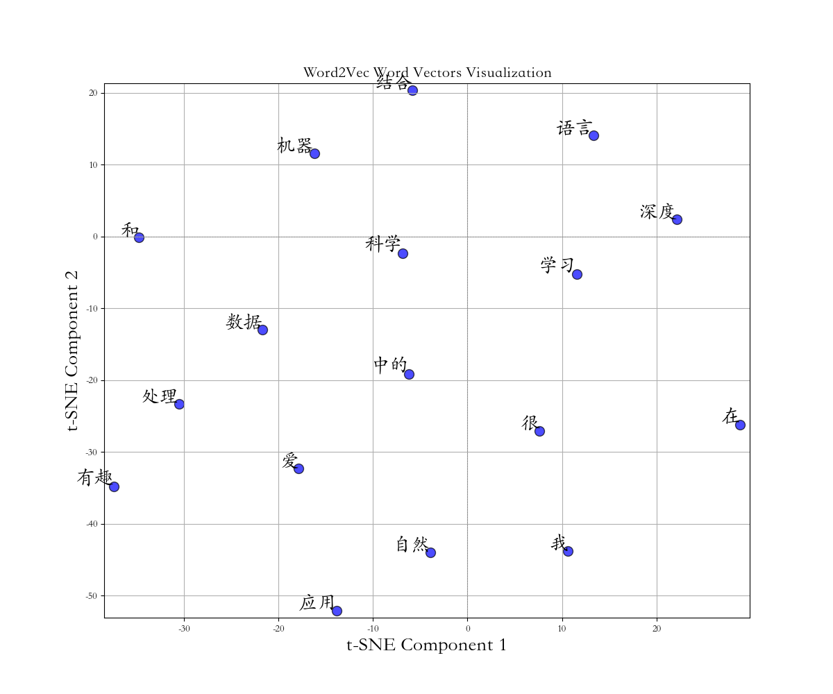
python
model = Word2Vec(
    sentences,         # 输入文本,是一个由句子组成的列表,必须提供
    vector_size=100,  # 每个词表示为100维的向量
    window=5,         # 训练时考虑中心词前后各5个上下文词
    min_count=1,      # 最低词频,只出现1次以上的词会被保留
    sg=1             # 模型类型:1=Skip-gram, 0=CBOW
)
2.2 GloVe
GloVe(Global Vectors for Word Representation)结合了全局矩阵分解 的优势(如LSA),局部上下文窗口 的优势(如Word2Vec),基本假设:共现概率比能更好地捕捉语义信息。
数学原理
- 共现矩阵
设XijX_{ij}Xij表示词jjj出现在词iii上下文中的次数,构建共现矩阵XXX。 - 损失函数
GloVe的目标是学习词向量wi\mathbf{w}_iwi和w~j\mathbf{\tilde{w}}_jw~j,使得:
wi⊤w~j+bi+b~j=logXij \mathbf{w}_i^{\top} \mathbf{\tilde{w}}_j + b_i + \tilde{b}j = \log X{ij} wi⊤w~j+bi+b~j=logXij
其中bib_ibi和b~j\tilde{b}_jb~j是偏置项。 - 加权最小二乘目标函数
J=∑i,j=1Vf(Xij)(wi⊤w~j+bi+b~j−logXij)2 J = \sum_{i,j=1}^{V} f(X_{ij}) \left( \mathbf{w}_i^{\top} \mathbf{\tilde{w}}_j + b_i + \tilde{b}j - \log X{ij} \right)^2 J=i,j=1∑Vf(Xij)(wi⊤w~j+bi+b~j−logXij)2
其中f(x)f(x)f(x)是加权函数,用于减少高频词的影响:
f(x)={(x/xmax)αif x<xmax1otherwise f(x) = \begin{cases} (x/x_{\max})^\alpha & \text{if } x < x_{\max} \\ 1 & \text{otherwise} \end{cases} f(x)={(x/xmax)α1if x<xmaxotherwise
通常xmax=100x_{\max} = 100xmax=100,α=3/4\alpha = 3/4α=3/4。
模型应用
python
import gensim.downloader as api
import matplotlib
import matplotlib.pyplot as plt
import numpy as np
from sklearn.manifold import TSNE

# 设置字体和负号显示
matplotlib.rcParams['axes.unicode_minus'] = False
matplotlib.rcParams['font.family'] = 'Kaiti SC'

# 下载 GloVe 模型
model = api.load("glove-wiki-gigaword-50")
print(f"✓ 模型加载完成!词汇表大小: {len(model)}")

# 获取特定词的词向量
word = "computer"
if word in model:
    print(f"\n'{word}' 的词向量(前5维): {model[word][:5]}")

# 查找相似词
test_words = ["king", "paris", "car", "happy"]
for word in test_words:
    if word in model:
        result = model.most_similar(word, topn=3)
        print(f"\n与 '{word}' 最相似的词:")
        for similar, score in result:
            print(f"  {similar}: {score:.4f}")

# 词类比
print("\n词类比任务:")
print("king - man + woman = ?")
result = model.most_similar(positive=["king", "woman"], negative=["man"], topn=3)
for word, score in result:
    print(f"  {word}: {score:.4f}")

# 简单可视化
words = ["king", "queen", "man", "woman", "boy", "girl",
         "paris", "london", "france", "england"]
vectors = []
labels = []
for word in words:
    if word in model:
        vectors.append(model[word])
        labels.append(word)

vectors = np.array(vectors)
if len(vectors) > 1:
    tsne = TSNE(n_components=2, random_state=42, perplexity=min(5, len(vectors) - 1))
    vectors_2d = tsne.fit_transform(vectors)

    # 可视化
    plt.figure(figsize=(10, 8))
    plt.scatter(vectors_2d[:, 0], vectors_2d[:, 1], s=100, alpha=0.7)

    for i, word in enumerate(labels):
        plt.annotate(
            word,
            xy=(vectors_2d[i, 0], vectors_2d[i, 1]),
            xytext=(5, 5),
            textcoords='offset points',
            fontsize=20  # 设置字体大小为20
        )

    plt.title("GloVe 词向量可视化", fontsize=20)
    plt.xlabel("t-SNE 维度 1", fontsize=20)
    plt.ylabel("t-SNE 维度 2", fontsize=20)
    plt.grid(True, alpha=0.3)
    plt.tight_layout()
    plt.show()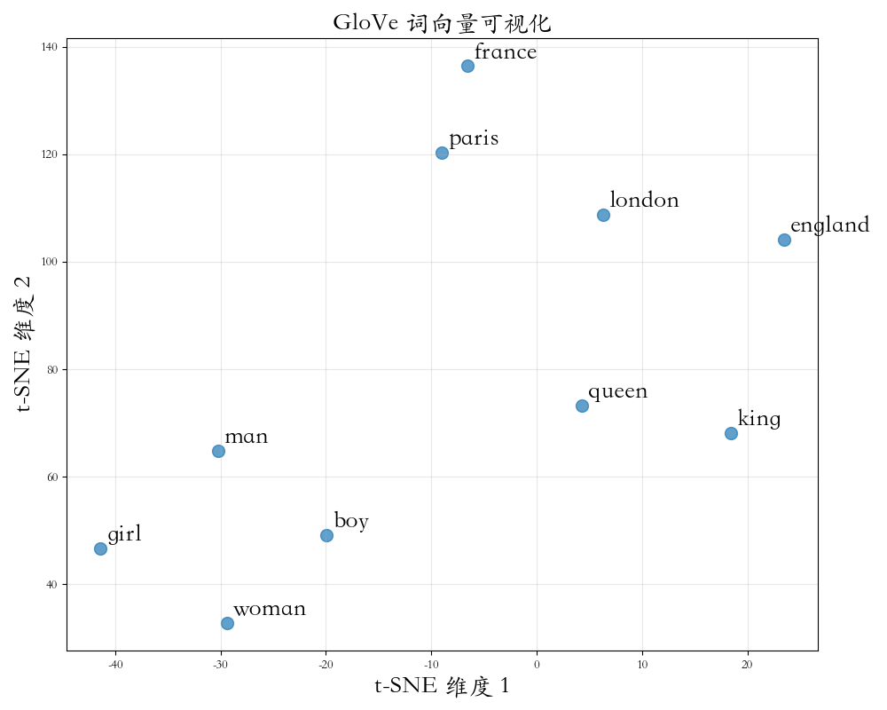
python
✓ 模型加载完成!词汇表大小: 400000

'computer' 的词向量(前5维): [ 0.079084 -0.81504   1.7901    0.91653   0.10797 ]

与 'king' 最相似的词:
  prince: 0.8236
  queen: 0.7839
  ii: 0.7746

与 'paris' 最相似的词:
  prohertrib: 0.8611
  france: 0.8025
  brussels: 0.7796

与 'car' 最相似的词:
  truck: 0.9209
  cars: 0.8870
  vehicle: 0.8834

与 'happy' 最相似的词:
  'm: 0.9142
  everyone: 0.8976
  everybody: 0.8965

词类比任务:
king - man + woman = ?
  queen: 0.8524
  throne: 0.7664
  prince: 0.7592
三、上下文表示时代
上下文表示时代标志着自然语言处理从静态词向量向动态上下文相关表示的转变。这个时代的核心突破是模型能够根据上下文为同一个词生成不同的向量表示,彻底解决了一词多义问题。
3.1 ELMo:一词多义的开端
ELMo(Embeddings from Language Models)首次实现了真正的上下文相关词向量。它的核心思想是:同一个词在不同上下文中应该有不同的向量表示。
技术原理
- 双向语言模型:通过两个独立的LSTM分别学习前向和后向的语言模型
python
# 前向LSTM: 从左到右预测下一个词
# 后向LSTM: 从右到左预测前一个词

# 前向语言模型: P(w1, w2, ..., wN) = ∏ P(wi | w1, ..., wi-1)
# 后向语言模型: P(w1, w2, ..., wN) = ∏ P(wi | wi+1, ..., wN)- 多层表示融合:ELMo 使用了多层 LSTM,每层捕获不同级别的语言信息
- 底层:句法信息(词性、语法结构)
- 中层:句法语义的过渡层
- 高层:语义信息
最终的词向量是各层表示的加权和:
ELMok=γ∑j=0Lsjhk,j \text{ELMo}k = \gamma \sum{j=0}^{L} s_j h_{k,j} ELMok=γj=0∑Lsjhk,j
模型架构
python
输入句子: "He played the piano and basketball."
ELMo处理流程:
1. 词嵌入层: 获取每个词的静态向量
2. 前向LSTM: 从左到右处理序列
3. 后向LSTM: 从右到左处理序列
4. 多层融合: 结合各层表示
5. 输出: 每个词的上下文相关向量
"play"在不同上下文中的不同表示:
- "play the piano" → 音乐相关的向量
- "play basketball" → 运动相关的向量
3.2 BERT:双向 Transformer
BERT(Bidirectional Encoder Representations from Transformers)基于Transformer编码器,通过掩码语言模型 和下一句预测任务进行预训练,学习深度双向的语言表示。
技术原理
- 掩码语言模型
python
# 随机掩盖输入序列中的15%的词
# 其中:80%替换为[MASK],10%替换为随机词,10%保持不变
# 目标:预测被掩盖的词

原始句子: "The cat sat on the mat."
掩盖后:   "The [MASK] sat on the mat."
目标: 预测"cat"- 下一句预测
python
# 判断两个句子是否连续
输入: [CLS] 句子A [SEP] 句子B [SEP]
标签: 1(连续)或0(不连续)

示例:
句子A: "The cat sat on the mat."
句子B: "It was sleeping peacefully."
标签: 1(连续)

句子A: "The cat sat on the mat."
句子B: "The weather is nice today."
标签: 0(不连续)
模型架构
python
输入: [CLS] 我 爱 自然 语言 处理 [SEP]
      ↓ Token Embedding
      ↓ Segment Embedding
      ↓ Position Embedding
      ↓
    Transformer编码器 × 12/24层
      ↓
输出: 每个位置的上下文相关向量
使用示例:文本相似度分析
python
import matplotlib
import matplotlib.pyplot as plt
import numpy as np
import torch
from sklearn.manifold import TSNE
from transformers import BertTokenizer, BertModel

# 设置中文字体
matplotlib.rcParams['axes.unicode_minus'] = False
matplotlib.rcParams['font.family'] = 'Kaiti SC'

# 加载预训练BERT模型和分词器
print("加载BERT模型...")
tokenizer = BertTokenizer.from_pretrained('bert-base-chinese')
model = BertModel.from_pretrained('bert-base-chinese')
model.eval()  # 设置为评估模式
print("模型加载完成!")

# 准备对比句子,包含语义相近和差异大的情况
sentences = [
    "我热爱音乐",  # 0: 爱
    "我喜欢读书",  # 1: 喜
    "我很爱好运动",  # 2: 爱
    "银行办理业务",  # 3: 行
    "他在行走",  # 4: 行
    "旅行行程安排",  # 5: 行
    "这个苹果很好吃",  # 6: 苹
    "苹果公司发布新手机",  # 7: 苹
    "他打篮球",  # 8: 打
    "我打电话",  # 9: 打
    "他打人",  # 10: 打
]

# 处理输入
inputs = tokenizer(sentences, padding=True, truncation=True, return_tensors="pt")

# 获取BERT表示
with torch.no_grad():
    outputs = model(**inputs)

last_hidden_states = outputs.last_hidden_state
print(f"批次大小: {last_hidden_states.shape[0]}")
print(f"最大序列长度: {last_hidden_states.shape[1]}")
print(f"隐藏维度: {last_hidden_states.shape[2]}")

# 分析每个句子,找到目标字的位置
target_chars = ['爱', '行', '苹', '打']  # 要分析的目标字
char_positions = {char: [] for char in target_chars}

for i, sent in enumerate(sentences):
    # 获取token
    tokens = tokenizer.tokenize(sent)

    # 找到目标字的位置
    for char in target_chars:
        if char in sent:
            # 找到对应的token位置
            token_pos = None
            for j, token in enumerate(tokens):
                if char in token:
                    token_pos = j
                    break
            if token_pos is not None:
                char_positions[char].append((i, token_pos, sent))

# 收集所有目标字的向量
all_vectors = []
all_labels = []
all_chars = []
all_sentences = []  # 用于存储句子

for char, positions in char_positions.items():
    for sent_idx, token_idx, sent in positions:
        vector = last_hidden_states[sent_idx, token_idx, :].numpy()
        all_vectors.append(vector)
        all_labels.append(sent)
        all_chars.append(char)
        all_sentences.append(sent)  # 存储句子

if len(all_vectors) > 1:
    all_vectors = np.array(all_vectors)

    # 使用t-SNE降维到2D
    tsne = TSNE(n_components=2, random_state=42, perplexity=min(5, len(all_vectors) - 1))
    vectors_2d = tsne.fit_transform(all_vectors)

    # 创建可视化
    plt.figure(figsize=(18, 10))

    # 为不同字使用不同颜色和标记
    char_colors = {'爱': '#FF6B6B', '行': '#4ECDC4', '苹': '#45B7D1', '打': '#96CEB4'}
    char_markers = {'爱': 'o', '行': 's', '苹': '^', '打': 'D'}
    char_sizes = {'爱': 200, '行': 180, '苹': 220, '打': 160}

    # 创建散点图
    for char in target_chars:
        # 筛选当前字的点
        indices = [i for i, c in enumerate(all_chars) if c == char]
        if indices:
            x_coords = [vectors_2d[i, 0] for i in indices]
            y_coords = [vectors_2d[i, 1] for i in indices]
            labels = [all_labels[i] for i in indices]

            # 绘制点
            plt.scatter(
                x_coords, y_coords,
                s=char_sizes[char],
                alpha=0.8,
                c=char_colors[char],
                marker=char_markers[char],
                edgecolors='black',
                linewidth=1.5,
                label=f"字'{char}'"
            )

            # 添加标签,显示字和句子
            for i, idx in enumerate(indices):
                plt.annotate(
                    f"{all_chars[idx]}: {all_sentences[idx]}",  # 显示字和句子
                    xy=(vectors_2d[idx, 0], vectors_2d[idx, 1]),
                    xytext=(8, 8),
                    textcoords='offset points',
                    fontsize=20,
                    fontweight='bold',
                    color=char_colors[char],
                    bbox=dict(
                        boxstyle="round,pad=0.3",
                        facecolor='white',
                        alpha=0.7,
                        edgecolor=char_colors[char],
                        linewidth=1
                    )
                )

    # 美化图形
    plt.title("BERT词向量t-SNE可视化(相同字在不同上下文)",
              fontsize=18, fontweight='bold', pad=20, color='#2C3E50')
    plt.xlabel("t-SNE维度 1", fontsize=14, fontweight='semibold', color='#34495E')
    plt.ylabel("t-SNE维度 2", fontsize=14, fontweight='semibold', color='#34495E')

    # 添加网格
    plt.grid(True, alpha=0.3, linestyle='--', linewidth=0.5)

    # 添加图例
    plt.legend(loc='best', fontsize=12, framealpha=0.9, shadow=True)

    # 添加说明文本
    plt.figtext(0.5, 0.01,
                "• 每个点代表一个汉字在特定上下文中的向量表示\n"
                "• 相同颜色的点表示同一个汉字\n"
                "• 点之间的距离表示语义相似度(越近越相似)",
                ha="center", fontsize=11,
                bbox=dict(boxstyle="round,pad=0.8", facecolor="lightyellow", alpha=0.7))

    plt.tight_layout(rect=[0, 0.05, 1, 0.97])
    plt.savefig('bert_word_vectors_tsne.png', dpi=300, bbox_inches='tight', facecolor='white')
    plt.show()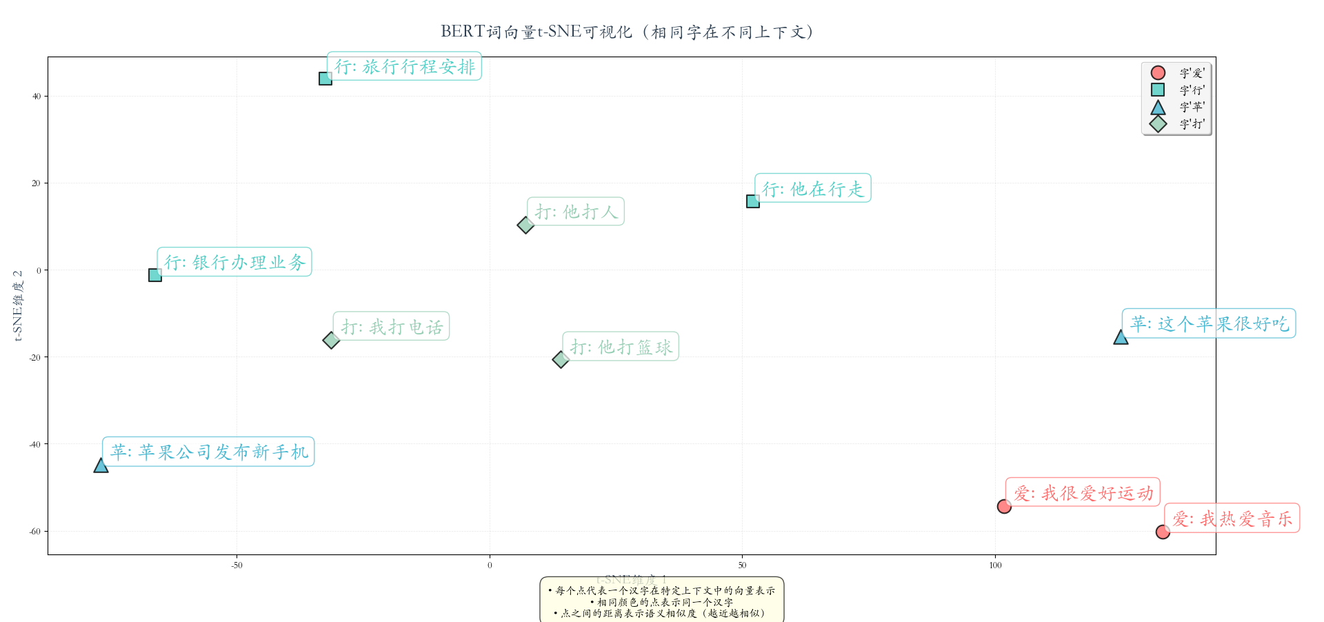
使用示例: 训练文本情感分类模型
python
import torch
import torch.nn as nn
import torch.optim as optim
from sklearn.model_selection import train_test_split
from torch.utils.data import DataLoader, Dataset
from transformers import BertTokenizer, BertForSequenceClassification

# 1. 准备数据
data = {
    'text': [
        # 正面评价 (1-25)
        "这部电影很好看,情节紧凑,演员演技在线",
        "这个产品很好用,质量超出预期,非常满意",
        "服务态度很好,耐心解答问题,体验很棒",
        "物流速度很快,包装完好无损,值得表扬",
        "性价比很高,物超所值,会推荐给朋友",
        "操作简单方便,界面友好,适合新手使用",
        "客服回复及时,解决问题效率高,点个赞",
        "外观设计漂亮,做工精细,很有质感",
        "功能强大实用,满足所有需求,非常好用",
        "送货上门及时,快递员服务态度很好",
        "价格实惠公道,品质却不打折,很棒",
        "使用效果明显,确实有效果,很惊喜",
        "售后服务到位,很有保障,买得放心",
        "食材新鲜美味,口感很好,下次还会来",
        "学习资源丰富,讲解清晰,收获很大",
        "环境干净整洁,氛围舒适,适合放松",
        "性能稳定流畅,运行速度快,不卡顿",
        "包装精美用心,送礼很有面子",
        "安装简单快捷,说明书清晰易懂",
        "声音效果震撼,视听体验一流",
        "续航能力强,用一整天都没问题",
        "画面清晰细腻,色彩还原真实",
        "界面设计美观,交互体验顺畅",
        "内容质量很高,干货满满,受益匪浅",
        "响应速度快,处理问题专业高效",

        # 负面评价 (26-50)
        "这个电影很无聊,剧情拖沓,看不下去",
        "质量很差,用了两天就坏了,不推荐",
        "服务态度很差,问什么都不耐烦",
        "物流超级慢,等了一周才到货",
        "价格虚高,完全不值这个价钱",
        "操作复杂难懂,根本不会用",
        "客服完全不回复,像机器人一样",
        "外观有瑕疵,做工粗糙,很失望",
        "功能太少,根本不够用,很差劲",
        "快递乱扔包裹,包装都破损了",
        "性价比极低,花钱买教训",
        "没有任何效果,纯粹浪费钱",
        "根本没有售后,出问题没人管",
        "食材不新鲜,味道很奇怪,难吃",
        "内容空洞无物,学不到东西",
        "环境脏乱差,待不下去想走",
        "经常死机卡顿,用得心烦",
        "包装简陋寒酸,像地摊货",
        "安装复杂困难,搞了半天没装好",
        "音质很差,杂音很多,听不清",
        "续航太差,用两小时就没电",
        "画面模糊不清,看着眼睛疼",
        "界面混乱难用,找不到功能",
        "内容质量低下,错误百出",
        "反应迟钝缓慢,效率低下"
    ],
    'label': [1, 1, 1, 1, 1, 1, 1, 1, 1, 1, 1, 1, 1, 1, 1, 1, 1, 1, 1, 1, 1, 1, 1, 1, 1, 0, 0, 0, 0, 0, 0, 0, 0, 0, 0,
              0, 0, 0, 0, 0, 0, 0, 0, 0, 0, 0, 0, 0, 0, 0]  # 1: 正面,0: 负面
}

# 2. 数据分割
train_texts, val_texts, train_labels, val_labels = train_test_split(
    data['text'], data['label'], test_size=0.33, random_state=42
)

print(f"训练集: {train_texts}")
print(f"验证集: {val_texts}")

# 3. 加载分词器
tokenizer = BertTokenizer.from_pretrained('bert-base-chinese')


# 4. 创建Dataset
class SentimentDataset(Dataset):
    def __init__(self, texts, labels, tokenizer, max_len=128):
        self.texts = texts
        self.labels = labels
        self.tokenizer = tokenizer
        self.max_len = max_len

    def __len__(self):
        return len(self.texts)

    def __getitem__(self, idx):
        text = str(self.texts[idx])
        label = self.labels[idx]

        encoding = self.tokenizer.encode_plus(
            text,
            add_special_tokens=True,
            max_length=self.max_len,
            padding='max_length',
            truncation=True,
            return_attention_mask=True,
            return_tensors='pt'
        )

        return {
            'input_ids': encoding['input_ids'].flatten(),
            'attention_mask': encoding['attention_mask'].flatten(),
            'labels': torch.tensor(label, dtype=torch.long)
        }


# 5. 创建数据集和数据加载器
train_dataset = SentimentDataset(train_texts, train_labels, tokenizer)
val_dataset = SentimentDataset(val_texts, val_labels, tokenizer)

train_loader = DataLoader(train_dataset, batch_size=2, shuffle=True)
val_loader = DataLoader(val_dataset, batch_size=2)

# 6. 加载模型
model = BertForSequenceClassification.from_pretrained(
    'bert-base-chinese',
    num_labels=2
)

# 7. 训练设置
device = torch.device('mps' if torch.mps.is_available() else 'cpu')
model.to(device)
optimizer = optim.AdamW(model.parameters(), lr=2e-5)
loss_fn = nn.CrossEntropyLoss()

# 8. 训练循环
print("\n开始训练...")
epochs = 15

for epoch in range(epochs):
    # 训练
    model.train()
    total_loss = 0

    for batch in train_loader:
        optimizer.zero_grad()

        input_ids = batch['input_ids'].to(device)
        attention_mask = batch['attention_mask'].to(device)
        labels = batch['labels'].to(device)

        outputs = model(input_ids, attention_mask=attention_mask, labels=labels)
        loss = outputs.loss
        total_loss += loss.item()

        loss.backward()
        optimizer.step()

    # 验证
    model.eval()
    correct = 0
    total = 0

    with torch.no_grad():
        for batch in val_loader:
            input_ids = batch['input_ids'].to(device)
            attention_mask = batch['attention_mask'].to(device)
            labels = batch['labels'].to(device)

            outputs = model(input_ids, attention_mask=attention_mask)
            predictions = torch.argmax(outputs.logits, dim=-1)

            correct += (predictions == labels).sum().item()
            total += labels.size(0)

    val_acc = correct / total
    print(f"Epoch {epoch + 1}/{epochs}: Loss={total_loss / len(train_loader):.4f}, Val Acc={val_acc:.4f}")

# 9. 保存模型
model.save_pretrained('./simple_sentiment_model')
tokenizer.save_pretrained('./simple_sentiment_model')
print(f"\n模型已保存到: ./simple_sentiment_model")


# 10. 预测函数
def predict(text, model_path='./simple_sentiment_model'):
    model = BertForSequenceClassification.from_pretrained(model_path)
    tokenizer = BertTokenizer.from_pretrained(model_path)

    model.eval()

    inputs = tokenizer(text, return_tensors='pt', truncation=True, max_length=128)

    with torch.no_grad():
        outputs = model(**inputs)
        probs = torch.nn.functional.softmax(outputs.logits, dim=-1)

    return probs[0].numpy()


# 测试
test_texts = ["这个产品很不错", "这个服务很糟糕"]
for text in test_texts:
    probs = predict(text)
    sentiment = "正面" if probs[1] > probs[0] else "负面"
    print(f"\n文本: {text}")
    print(f"预测: {sentiment}")
    print(f"负面概率: {probs[0]:.4f}, 正面概率: {probs[1]:.4f}")
python
文本: 这个产品很不错
预测: 正面
负面概率: 0.0019, 正面概率: 0.9981

文本: 这个服务很糟糕
预测: 负面
负面概率: 0.9605, 正面概率: 0.0395
3.3 GPT 系列:自回归生成模型
GPT(Generative Pre-trained Transformer)系列基于Transformer解码器,通过自回归语言建模进行预训练,具有强大的文本生成能力。
| 版本 | 发布时间 | 参数量 | 关键技术 | 主要突破 |
|---|---|---|---|---|
| GPT-1 | 2018.6 | 117M | Transformer解码器 | 预训练+微调范式 |
| GPT-2 | 2019.2 | 1.5B | 更大模型+更多数据 | 零样本学习能力 |
| GPT-3 | 2020.5 | 175B | 规模扩展 | 上下文学习、思维链 |
| GPT-4 | 2023.3 | ~1.7T | MoE架构、多模态 | 更强推理、多模态理解 |
| GPT-4o | 2024.5 | 约500B量级 | 原生多模态(文本、图像、音频) | 端到端多模态,响应速度更快,成本降低至GPT-4的1/3 |
| o1 / o3 系列 | 2024.9 | 未明确 | 推理优化架构 | 专注于深度推理和复杂问题解决,在数学、科学等领域表现突出 |
| GPT-4.5 | 2025.2(研究预览) | 未明确(约5.7T) | 过渡性升级 | 作为GPT-4o的增强版推出 |
| GPT-5 | 2025.8 | 52万亿(标准版) | "Transformer-深度递归单元"混合架构 | 统一系统,智能调度子模型,在编程、数学、视觉感知等领域性能大幅提升,并向免费用户有限开放 |
模型架构
python
GPT 基于 Transformer 解码器:
1. 自注意力层(带掩码,只能看前面)
2. 前馈神经网络
3. 层归一化和残差连接
4. 重复 N 次(GPT-3: 96层)

训练目标:最大化似然函数
L = Σ log P(wi | w1, w2, ..., wi-1)