【GA-Net】《GA-Net: Guided Aggregation Net for End-to-end Stereo Matching》

CVPR-2019

github：https://github.com/feihuzhang/GANet

文章目录

[1、Background and Motivation](#1、Background and Motivation)
[2、Related Work](#2、Related Work)
[3、Advantages / Contributions](#3、Advantages / Contributions)
4、Method
- [4.1、Network Architecture](#4.1、Network Architecture)
- [4.2、Guided Aggregation Layers](#4.2、Guided Aggregation Layers)
- [4.3、Loss Function](#4.3、Loss Function)
5、Experiments
- [5.1、Datasets and Metrics](#5.1、Datasets and Metrics)
- [5.2、Ablation Study](#5.2、Ablation Study)
- [5.3、Effects of Guided Aggregations](#5.3、Effects of Guided Aggregations)
- [5.4、Comparisons with SGMs and 3D Convolutions](#5.4、Comparisons with SGMs and 3D Convolutions)
- [5.5、Complexity and Realtime Models](#5.5、Complexity and Realtime Models)
- [5.6、Evaluations on Benchmarks](#5.6、Evaluations on Benchmarks)
[6、Conclusion（own） / Future work](#6、Conclusion（own） / Future work)

1、Background and Motivation

立体匹配（Stereo Matching）是计算机视觉中的经典任务，旨在从一对左右视图图像中估计每个像素的视差（disparity），从而恢复三维场景结构。该任务在自动驾驶、机器人导航、增强现实等领域具有广泛应用。

传统立体匹配流程通常包含三个步骤：

特征提取（feature extraction ）与代价计算（matching cost computation）：对左右图像提取特征并构建初始匹配代价；
代价聚合（Cost Aggregation）：对初始代价进行平滑和优化，以抑制噪声、填补纹理缺失区域；
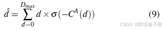
视差回归或优化（disparity prediction）：从聚合后的代价体中预测最终视差图。

尽管深度学习方法在特征提取方面取得了巨大成功，但 cost aggregation 仍是决定整体性能的关键瓶颈。

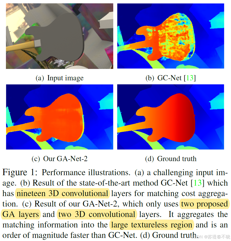
早期深度方法（如 MC-CNN）仍依赖传统聚合策略（如 semi-global matching（SGM）或滤波，are not differentiable and cannot be easily trained in an end-to-end manner），而端到端模型（如 GC-Net、PSMNet）则采用3D 卷积对代价体进行聚合------虽然有效，却带来高昂的计算和内存开销（复杂度为 O ( K 3 C N ) O(K^3CN) O(K3CN)，其中 K 为卷积核大小，C 为通道数，N 为体素数量）。

作者观察到：

3D 卷积效率低下：为了处理高分辨率代价体，现有方法常通过下采样减少计算量，但这会损失细节，尤其在薄结构和边缘处表现不佳。
传统聚合方法不可微：经典的半全局匹配（SGM）和引导滤波虽高效鲁棒，但因其非可微性，无法嵌入端到端训练框架。

因此，能否设计一种既高效又可微的代价聚合机制，替代昂贵的 3D 卷积？

作者提出 Guided Aggregation Net（GAnet），更好更高效的优化 cost aggregation 模块

The cost volume C is formed of matching costs at each pixel's location for each candidate disparity value d.

（1）Deep Neural Networks for Stereo Matching

DispNet (2016)：首个端到端立体匹配网络，但未显式建模代价聚合。
GC-Net (2017)：引入 3D 卷积进行代价聚合，实现端到端训练。
PSMNet (2018)：结合金字塔特征与堆叠沙漏结构，使用多达 25 层 3D 卷积，精度提升但计算成本剧增。

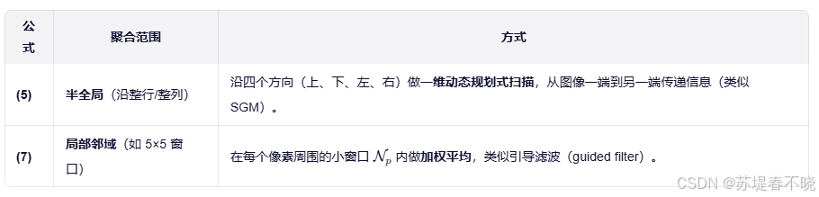
（2）Cost Aggregation

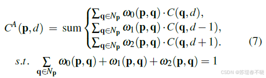
Local Cost Aggregation：如引导滤波（Guided Filter）、双边滤波，在局部窗口内加权平均代价。

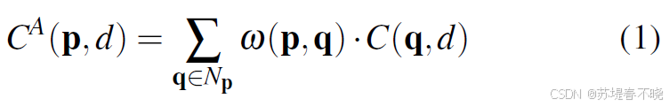
pixel's location p = (x,y)

neighborhoods q ∈ N p \in N_p ∈Np（local region）

C ( p , d ) C(p,d) C(p,d)，the matching cost at location p for candidate disparity d

C A ( p , d ) C^A(p,d) CA(p,d)，aggregated matching cost

Different image filters can be used to produce the guided filter weights w w w

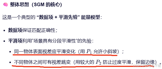
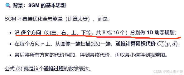
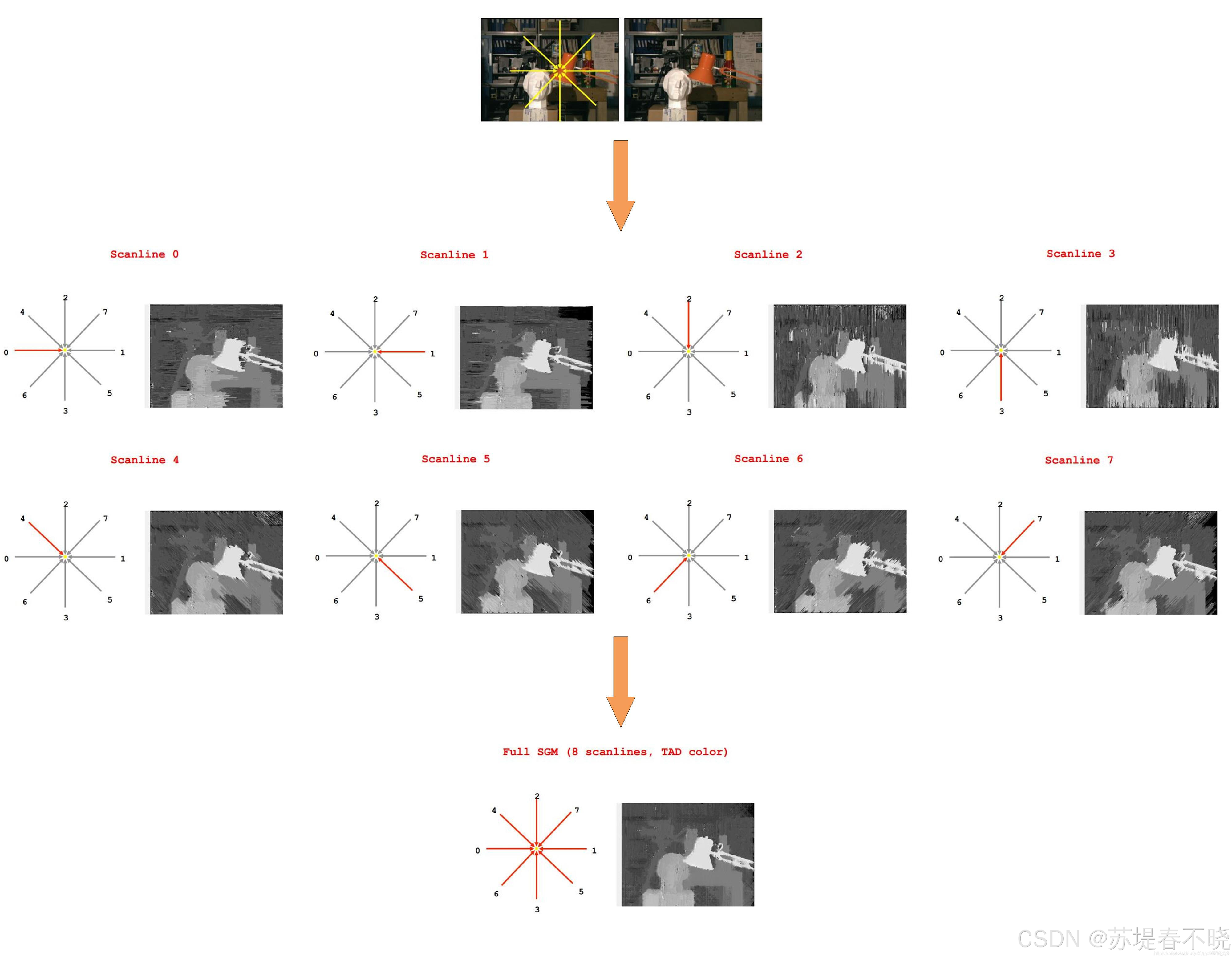
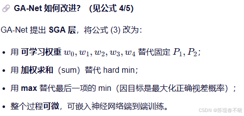
Semi-Global Matching（SGM）：沿多个方向动态规划聚合代价，兼顾全局一致性与边界保持。然而，这些方法均不可微，难以与神经网络联合优化。

formulated into one energy function E(D)

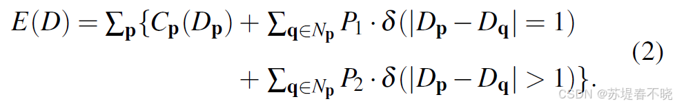
minimizes the energy E ( D ) E(D) E(D)

constant penalty P1

larger constant penalty P2

disparity map D

δ \delta δ(condition)：指示函数，条件为真时值为 1，否则为 0；

第一项数据项，鼓励选择匹配代价低的视差

第二项平滑项（小跳跃惩罚），允许相邻像素视差有小幅变化（如斜面），但要付出一定代价。

第三项平滑项（大跳跃惩罚），强烈抑制非边缘区域的视差突变，但允许真实物体边界存在不连续（因为 P2 虽大，若数据项 C 足够强仍可保留边缘）。

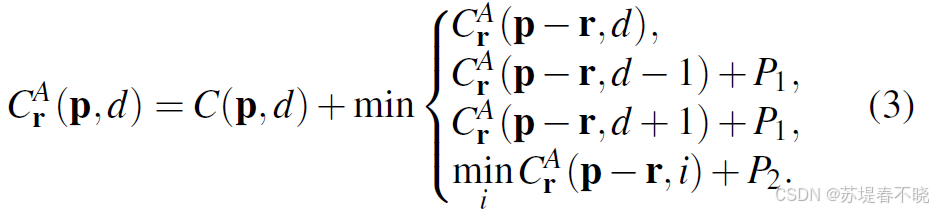
P1 和 P2 是手动设定的参数

r r r unit direction vector

论文阅读 GA-Net: Guided Aggregation Net for End-to-end Stereo Matching

3、Advantages / Contributions

GA-Net 优化 cost aggregation 模块，提出两种新型可微层，速度精度显著优于 3D 卷积：

半全局引导聚合层（SGA, Semi-Global Aggregation）：occlusions, large textureless/reflective regions
局部引导聚合层（LGA, Local Guided Aggregation）：thin structures

4、Method

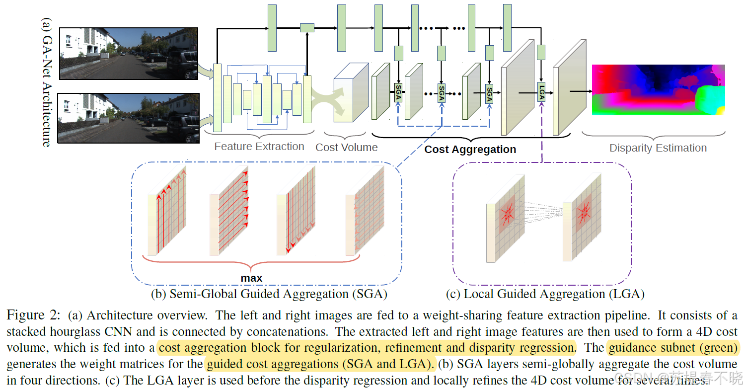
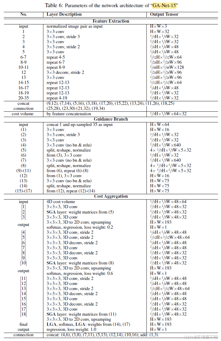
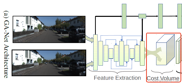
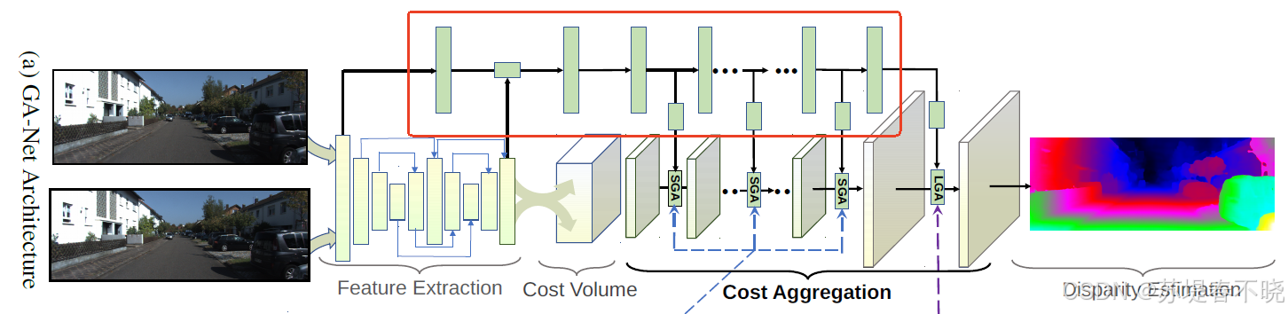
4.1、Network Architecture

python 复制代码

    def forward(self, x, y):
        g = self.conv_start(x)  # torch.Size([1, 32, 384, 1248])->torch.Size([1, 32, 384, 1248])	
        x = self.feature(x)  # 1/3 torch.Size([1, 32, 128, 416])

        rem = x 
        x = self.conv_x(x)  # 1/3 torch.Size([1, 32, 128, 416])

        y = self.feature(y)
        y = self.conv_y(y)  # 1/3 torch.Size([1, 32, 128, 416])

        x = self.cv(x,y)  # torch.Size([1, 64, 65, 128, 416]) concatenation cost volume 192/3 + 1 = 65

        x1 = self.conv_refine(rem)  # torch.Size([1, 32, 128, 416])
        x1 = F.interpolate(x1, [x1.size()[2]*3,x1.size()[3]*3], mode='bilinear', align_corners=False)
        x1 = self.bn_relu(x1)  # torch.Size([1, 32, 384, 1248])
        g = torch.cat((g, x1), 1)  # torch.Size([1, 64, 384, 1248])
        g = self.guidance(g)  # 9 个输出
        if self.training:
            disp0, disp1, disp2 = self.cost_agg(x, g)
            return disp0, disp1, disp2
        else:
            return self.cost_agg(x, g)

（1）feature extraction block（stacked hourglass network）

其中 self.feature 就是 feature extraction block 模块

python 复制代码

    def forward(self, x):
        x = self.conv_start(x)  # 1/3 torch.Size([1, 32, 128, 416])
        rem0 = x
        x = self.conv1a(x)  # 1/6 torch.Size([1, 48, 64, 208])
        rem1 = x
        x = self.conv2a(x)  # 1/12 torch.Size([1, 64, 32, 104])
        rem2 = x
        x = self.conv3a(x)  # 1/24 torch.Size([1, 96, 16, 52])
        rem3 = x
        x = self.conv4a(x)  # 1/48 torch.Size([1, 128, 8, 26])
        rem4 = x
        x = self.deconv4a(x, rem3)  # 1/24 torch.Size([1, 96, 16, 52])
        rem3 = x

        x = self.deconv3a(x, rem2)  # 1/12 torch.Size([1, 64, 32, 104])
        rem2 = x
        x = self.deconv2a(x, rem1)  # 1/6 torch.Size([1, 48, 64, 208])
        rem1 = x
        x = self.deconv1a(x, rem0)  # 1/3 torch.Size([1, 32, 128, 416])
        rem0 = x

        x = self.conv1b(x, rem1)  # 1/6 torch.Size([1, 48, 64, 208])
        rem1 = x
        x = self.conv2b(x, rem2)  # 1/12 torch.Size([1, 64, 32, 104])
        rem2 = x
        x = self.conv3b(x, rem3)  # 1/24 torch.Size([1, 96, 16, 52])
        rem3 = x
        x = self.conv4b(x, rem4)  # 1/48 torch.Size([1, 128, 8, 26])

        x = self.deconv4b(x, rem3)  # 1/24 torch.Size([1, 96, 16, 52])
        x = self.deconv3b(x, rem2)  # 1/12 torch.Size([1, 64, 32, 104])
        x = self.deconv2b(x, rem1)  # 1/6 torch.Size([1, 48, 64, 208])
        x = self.deconv1b(x, rem0)  # 1/3 torch.Size([1, 32, 128, 416])

        return x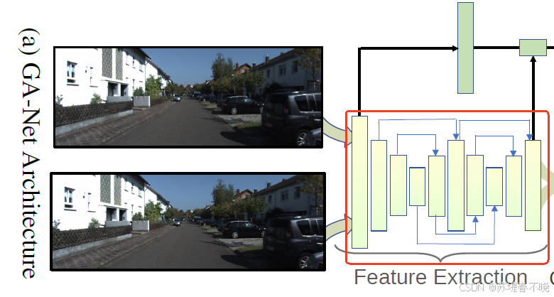

可以看到是有两个 hourglass network 的

（2）the cost aggregation

python 复制代码

x = self.cv(x,y)  # torch.Size([1, 64, 65, 128, 416]) concatenation cost volume 192/3 + 1 = 65

对应的实现

python 复制代码

class GetCostVolume(Module):
    def __init__(self, maxdisp):
        super(GetCostVolume, self).__init__()
        self.maxdisp = maxdisp + 1

    def forward(self, x, y):
        assert(x.is_contiguous() == True)
        with torch.cuda.device_of(x):
            num, channels, height, width = x.size()
            cost = x.new().resize_(num, channels * 2, self.maxdisp, height, width).zero_()
#            cost = Variable(torch.FloatTensor(x.size()[0], x.size()[1]*2, self.maxdisp,  x.size()[2],  x.size()[3]).zero_(), volatile= not self.training).cuda()
            for i in range(self.maxdisp):
                if i > 0 :
                    cost[:, :x.size()[1], i, :,i:]   = x[:,:,:,i:]
                    cost[:, x.size()[1]:, i, :,i:]   = y[:,:,:,:-i]
                else:
                    cost[:, :x.size()[1], i, :,:]   = x
                    cost[:, x.size()[1]:, i, :,:]   = y

            cost = cost.contiguous()
        return cost

就是常规的 concatenation cost construction

（3）the guidance subnet

公式 5 和公式 7 中的 weights 都是通过 guidance subnet learning 出来的

python 复制代码

 g = self.guidance(g)  # 9 个输出

concatenate 一些左图特征后作为输入

完整实现如下

python 复制代码

class Guidance(nn.Module):
    def __init__(self):
        super(Guidance, self).__init__()

        self.conv0 = BasicConv(64, 16, kernel_size=3, padding=1)
        self.conv1 = nn.Sequential(
            BasicConv(16, 32, kernel_size=5, stride=3, padding=2),
            BasicConv(32, 32, kernel_size=3, padding=1))

        self.conv2 = BasicConv(32, 32, kernel_size=3, padding=1)
        self.conv3 = BasicConv(32, 32, kernel_size=3, padding=1)

#        self.conv11 = Conv2x(32, 48)
        self.conv11 = nn.Sequential(BasicConv(32, 48, kernel_size=3, stride=2, padding=1),
                                    BasicConv(48, 48, kernel_size=3, padding=1))
        self.conv12 = BasicConv(48, 48, kernel_size=3, padding=1)
        self.conv13 = BasicConv(48, 48, kernel_size=3, padding=1)
        self.conv14 = BasicConv(48, 48, kernel_size=3, padding=1)

        self.weight_sg1 = nn.Conv2d(32, 640, (3, 3), (1, 1), (1, 1), bias=False)
        self.weight_sg2 = nn.Conv2d(32, 640, (3, 3), (1, 1), (1, 1), bias=False)
        self.weight_sg3 = nn.Conv2d(32, 640, (3, 3), (1, 1), (1, 1), bias=False)

        self.weight_sg11 = nn.Conv2d(48, 960, (3, 3), (1, 1), (1, 1), bias=False)
        self.weight_sg12 = nn.Conv2d(48, 960, (3, 3), (1, 1), (1, 1), bias=False)
        self.weight_sg13 = nn.Conv2d(48, 960, (3, 3), (1, 1), (1, 1), bias=False)
        self.weight_sg14 = nn.Conv2d(48, 960, (3, 3), (1, 1), (1, 1), bias=False)

        self.weight_lg1 = nn.Sequential(BasicConv(16, 16, kernel_size=3, padding=1),
                                        nn.Conv2d(16, 75, (3, 3), (1, 1), (1, 1) ,bias=False))
        self.weight_lg2 = nn.Sequential(BasicConv(16, 16, kernel_size=3, padding=1),
                                        nn.Conv2d(16, 75, (3, 3), (1, 1), (1, 1) ,bias=False))

    def forward(self, x):
        x = self.conv0(x)  # torch.Size([1, 64, 384, 1248])->torch.Size([1, 16, 384, 1248])
        rem = x
        x = self.conv1(x)  # 1/3 torch.Size([1, 32, 128, 416])
        sg1 = self.weight_sg1(x)  # 1/3 torch.Size([1, 640, 128, 416])
        x = self.conv2(x)  # 1/3 torch.Size([1, 32, 128, 416])
        sg2 = self.weight_sg2(x)  # 1/3 torch.Size([1, 640, 128, 416])
        x = self.conv3(x)  # 1/3 torch.Size([1, 32, 128, 416])
        sg3 = self.weight_sg3(x)  # torch.Size([1, 640, 128, 416])

        x = self.conv11(x)  # 1/6 torch.Size([1, 48, 64, 208])
        sg11 = self.weight_sg11(x)  # 1/6 torch.Size([1, 960, 64, 208])
        x = self.conv12(x)  # 1/6 torch.Size([1, 48, 64, 208])
        sg12 = self.weight_sg12(x)  # 1/6 torch.Size([1, 960, 64, 208])
        x = self.conv13(x)  # 1/6 torch.Size([1, 48, 64, 208])
        sg13 = self.weight_sg13(x)  # 1/6 torch.Size([1, 960, 64, 208])
        x = self.conv14(x)  # 1/6 torch.Size([1, 48, 64, 208])
        sg14 = self.weight_sg14(x)  # 1/6 torch.Size([1, 960, 64, 208])

        lg1 = self.weight_lg1(rem)  # torch.Size([1, 75, 384, 1248])
        lg2 = self.weight_lg2(rem)  # torch.Size([1, 75, 384, 1248])
       
        return dict([
            ('sg1', sg1),
            ('sg2', sg2),
            ('sg3', sg3),
            ('sg11', sg11),
            ('sg12', sg12),
            ('sg13', sg13),
            ('sg14', sg14),
            ('lg1', lg1),
            ('lg2', lg2)])

可以看到输出 feature 的 channel 都非常大，是为了后续 SGA 和 LGA 模块 split

4.2、Guided Aggregation Layers

guided aggregation (GA) strategies

semi-global guided aggregation layer (SGA)，a differentiable approximation of semi-global matching (SGM)，enables accurate estimations in occluded regions or large textureless/reflective regions
local guided aggregation layer(LGA)，cope with thin structures and object edges in order to recover the loss of details caused by down-sampling and up-sampling layers.

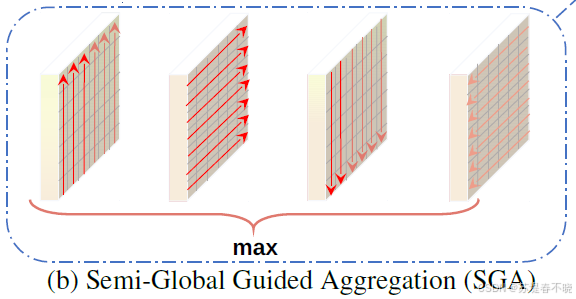
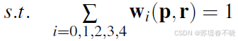
（1）Semi-Global Aggregation

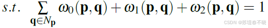
normalize the weights of the terms

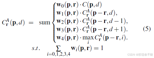
所有的 w w w 是通过 guidance subnet 来实现的

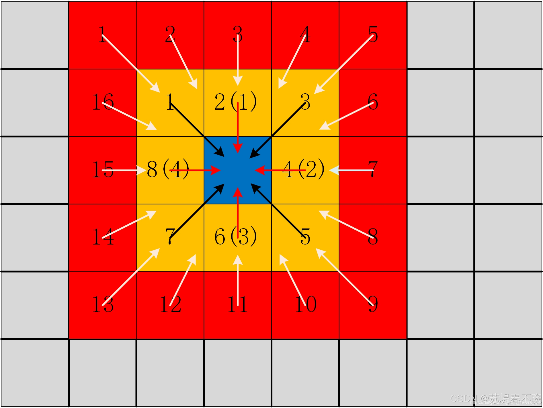
totally four directions (left, right, up and down)

namely r ∈ { ( 0 , 1 ) , ( 0 , − 1 ) , ( 1 , 0 ) , ( − 1 , 0 ) } r \in \{(0,1), (0,-1), (1,0), (-1,0)\} r∈{(0,1),(0,−1),(1,0),(−1,0)}

last maximum selection keeps the best message from only one direction.

cuda 源码中可以比较清晰的看到，每次比较一个方向的结果与当前最优值；保留更大的那个，并记录来自哪个方向（存入 mask），mask 用于反向传播

SGA layer can be repeated several times

cost aggregation 对应的 code

python 复制代码

class CostAggregation(nn.Module):
    def __init__(self, maxdisp=192):
        super(CostAggregation, self).__init__()
        self.maxdisp = maxdisp
        self.conv_start = BasicConv(64, 32, is_3d=True, kernel_size=3, padding=1, relu=False)

        self.conv1a = BasicConv(32, 48, is_3d=True, kernel_size=3, stride=2, padding=1)
        self.conv2a = BasicConv(48, 64, is_3d=True, kernel_size=3, stride=2, padding=1)
#        self.conv3a = BasicConv(64, 96, is_3d=True, kernel_size=3, stride=2, padding=1)

        self.deconv1a = Conv2x(48, 32, deconv=True, is_3d=True, relu=False)
        self.deconv2a = Conv2x(64, 48, deconv=True, is_3d=True)
#        self.deconv3a = Conv2x(96, 64, deconv=True, is_3d=True)

        self.conv1b = Conv2x(32, 48, is_3d=True)
        self.conv2b = Conv2x(48, 64, is_3d=True)
#        self.conv3b = Conv2x(64, 96, is_3d=True)

        self.deconv1b = Conv2x(48, 32, deconv=True, is_3d=True, relu=False)
        self.deconv2b = Conv2x(64, 48, deconv=True, is_3d=True)
#        self.deconv3b = Conv2x(96, 64, deconv=True, is_3d=True)
        self.deconv0b = Conv2x(8, 8, deconv=True, is_3d=True)
        
        self.sga1 = SGABlock(refine=True)
        self.sga2 = SGABlock(refine=True)
        self.sga3 = SGABlock(refine=True)

        self.sga11 = SGABlock(channels=48, refine=True)
        self.sga12 = SGABlock(channels=48, refine=True)
        self.sga13 = SGABlock(channels=48, refine=True)
        self.sga14 = SGABlock(channels=48, refine=True)

        self.disp0 = Disp(self.maxdisp)
        self.disp1 = Disp(self.maxdisp)
        self.disp2 = DispAgg(self.maxdisp)


    def forward(self, x, g):
        
        x = self.conv_start(x)  # 1/3 torch.Size([1, 64, 65, 128, 416])->torch.Size([1, 32, 65, 128, 416])
        x = self.sga1(x, g['sg1'])
        rem0 = x
       
        if self.training:
            disp0 = self.disp0(x)

        x = self.conv1a(x)
        x = self.sga11(x, g['sg11']) # torch.Size([1, 48, 33, 64, 208])
        rem1 = x
        x = self.conv2a(x)           # torch.Size([1, 64, 17, 32, 104])
        rem2 = x
#        x = self.conv3a(x)
#        rem3 = x

#        x = self.deconv3a(x, rem2)
#        rem2 = x
        x = self.deconv2a(x, rem1)   # torch.Size([1, 48, 33, 64, 208])
        x = self.sga12(x, g['sg12']) # torch.Size([1, 48, 33, 64, 208])
        rem1 = x
        x = self.deconv1a(x, rem0)   # torch.Size([1, 32, 65, 128, 416])
        x = self.sga2(x, g['sg2'])   # torch.Size([1, 32, 65, 128, 416])
        rem0 = x
        if self.training:
            disp1 = self.disp1(x)

        x = self.conv1b(x, rem1)      # torch.Size([1, 48, 33, 64, 208])
        x = self.sga13(x, g['sg13'])  # torch.Size([1, 48, 33, 64, 208])
        rem1 = x
        x = self.conv2b(x, rem2)      # torch.Size([1, 64, 17, 32, 104])
#        rem2 = x
#        x = self.conv3b(x, rem3)

#        x = self.deconv3b(x, rem2)
        x = self.deconv2b(x, rem1)   # torch.Size([1, 48, 33, 64, 208])
        x = self.sga14(x, g['sg14']) # torch.Size([1, 48, 33, 64, 208])
        x = self.deconv1b(x, rem0)   # torch.Size([1, 32, 65, 128, 416])
        x = self.sga3(x, g['sg3'])   # torch.Size([1, 32, 65, 128, 416])

        disp2 = self.disp2(x, g['lg1'], g['lg2'])  # torch.Size([1, 384, 1248])
        if self.training:
            return disp0, disp1, disp2
        else:
            return disp2

其中 SGABlock 的实现如下，可以看到 split 操作，split 成 5 份，后面 4 份是 4 个方向

python 复制代码

class SGABlock(nn.Module):
    def __init__(self, channels=32, refine=False):
        super(SGABlock, self).__init__()
        self.refine = refine
        if self.refine:
            self.bn_relu = nn.Sequential(BatchNorm3d(channels),
                                         nn.ReLU(inplace=True))
            self.conv_refine = BasicConv(channels, channels, is_3d=True, kernel_size=3, padding=1, relu=False)
#            self.conv_refine1 = BasicConv(8, 8, is_3d=True, kernel_size=1, padding=1)
        else:
            self.bn = BatchNorm3d(channels)
        self.SGA=SGA()
        self.relu = nn.ReLU(inplace=True)
    def forward(self, x, g):
        rem = x  # torch.Size([1, 32, 65, 128, 416]), g=torch.Size([1, 640, 128, 416]) 
        k1, k2, k3, k4 = torch.split(g, (x.size()[1]*5, x.size()[1]*5, x.size()[1]*5, x.size()[1]*5), 1) # torch.Size([1, 160, 128, 416])
        k1 = F.normalize(k1.view(x.size()[0], x.size()[1], 5, x.size()[3], x.size()[4]), p=1, dim=2)  #  torch.Size([1, 32, 5, 128, 416])
        k2 = F.normalize(k2.view(x.size()[0], x.size()[1], 5, x.size()[3], x.size()[4]), p=1, dim=2)  #  torch.Size([1, 32, 5, 128, 416])
        k3 = F.normalize(k3.view(x.size()[0], x.size()[1], 5, x.size()[3], x.size()[4]), p=1, dim=2)  #  torch.Size([1, 32, 5, 128, 416])
        k4 = F.normalize(k4.view(x.size()[0], x.size()[1], 5, x.size()[3], x.size()[4]), p=1, dim=2)  #  torch.Size([1, 32, 5, 128, 416])
        x = self.SGA(x, k1, k2, k3, k4)  # torch.Size([1, 32, 65, 128, 416])
        if self.refine:
            x = self.bn_relu(x)
            x = self.conv_refine(x)
        else:
            x = self.bn(x)
        assert(x.size() == rem.size())
        x += rem  # torch.Size([1, 32, 65, 128, 416])
        return self.relu(x)    
#        return self.bn_relu(x)

torch.nn.functional.normalize，默认是 L2 范式

对应的是公式中的该部分吗？

self.SGA 对应 cuda forward 源码 ~/GANet-master/libs/GANet/src/GANet_kernel.cu 如下

python 复制代码

// SGA（空间引导聚合）前向传播函数：对输入代价体沿四个方向（下、上、右、左）进行加权聚合，并取各方向最大响应作为输出
void sga_kernel_forward (
    at::Tensor input,           // 输入代价体，形状 [B, C, D, H, W]
    at::Tensor guidance_down,   // 向下方向的引导权重，形状 [B, C, K, H, W]（K 为聚合窗口大小）
    at::Tensor guidance_up,     // 向上方向的引导权重
    at::Tensor guidance_right,  // 向右方向的引导权重
    at::Tensor guidance_left,   // 向左方向的引导权重
    at::Tensor temp_out,        // 临时缓冲张量，用于存储中间聚合结果
    at::Tensor output,          // 最终输出张量，存储四方向最大响应
    at::Tensor mask             // 方向掩码，记录每个位置的最大值来自哪个方向（0=down,1=up,2=right,3=left）
) {
  
  // 获取输入张量各维度大小
  int num = input.size(0);     // batch size (B)
  int channel = input.size(1); // 通道数 (C)，通常为1
  int depth = input.size(2);   // 视差维度 (D)
  int height = input.size(3);  // 图像高度 (H)
  int width = input.size(4);   // 图像宽度 (W)
  int wsize = guidance_down.size(2); // 聚合窗口大小（如9）

  // 获取输出、临时缓冲、掩码的设备指针（GPU显存地址）
  float *top_data = output.data<float>();      // 最终输出指针
  float *top_temp = temp_out.data<float>();    // 临时工作区指针
  float *top_mask = mask.data<float>();        // 方向掩码指针

  // 获取输入和四个方向引导权重的只读指针
  const float *bottom_data = input.data<float>(); // 原始输入代价体
  const float *g0 = guidance_down.data<float>();
  const float *g1 = guidance_up.data<float>();
  const float *g2 = guidance_right.data<float>();
  const float *g3 = guidance_left.data<float>();

  // 计算用于水平方向（上下）聚合的线程配置参数
  int n = num * channel * width;                     // 每次处理的"列"元素总数（沿高度方向聚合）
  int threads = (n + CUDA_NUM_THREADS - 1) / CUDA_NUM_THREADS; // 启动的block数（向上取整）
  int N = input.numel();                             // 总元素数（B*C*D*H*W）

  // 【步骤1】向下方向聚合（从上到下扫描）
  // 将原始输入复制到临时缓冲区（确保每次聚合都从原始输入开始）
  cudaMemcpy(top_temp, bottom_data, sizeof(float) * N, cudaMemcpyDeviceToDevice);
  // 启动CUDA kernel：沿"向下"方向做加权聚合（使用g0引导权重）
  sga_down_forward<<<threads, CUDA_NUM_THREADS>>>(n, g0, height, width, depth, wsize, top_temp);
  // 将向下聚合结果暂存为当前最优输出
  cudaMemcpy(top_data, top_temp, sizeof(float) * N, cudaMemcpyDeviceToDevice);

  // 【步骤2】向上方向聚合（从下到上扫描）
  // 重新从原始输入复制到临时缓冲区
  cudaMemcpy(top_temp, bottom_data, sizeof(float) * N, cudaMemcpyDeviceToDevice);
  // 启动向上聚合kernel（使用g1）
  sga_up_forward<<<threads, CUDA_NUM_THREADS>>>(n, g1, height, width, depth, wsize, top_temp);
  // 与当前最优输出比较，逐元素取最大值，并更新mask（方向=1）
  Max<<<(N + CUDA_NUM_THREADS - 1) / CUDA_NUM_THREADS, CUDA_NUM_THREADS>>>(
      N, top_temp, top_data, top_mask, 1);

  // 【步骤3】向右方向聚合（从左到右扫描）
  // 更新线程配置：现在处理"行"（沿宽度方向聚合）
  n = num * channel * height;
  threads = (n + CUDA_NUM_THREADS - 1) / CUDA_NUM_THREADS;

  // 重新从原始输入复制
  cudaMemcpy(top_temp, bottom_data, sizeof(float) * N, cudaMemcpyDeviceToDevice);
  // 启动向右聚合kernel（使用g2）
  sga_right_forward<<<threads, CUDA_NUM_THREADS>>>(n, g2, height, width, depth, wsize, top_temp);
  // 与当前最优比较，取最大，更新mask（方向=2）
  Max<<<(N + CUDA_NUM_THREADS - 1) / CUDA_NUM_THREADS, CUDA_NUM_THREADS>>>(
      N, top_temp, top_data, top_mask, 2);

  // 【步骤4】向左方向聚合（从右到左扫描）
  // 重新从原始输入复制
  cudaMemcpy(top_temp, bottom_data, sizeof(float) * N, cudaMemcpyDeviceToDevice);
  // 启动向左聚合kernel（使用g3）
  sga_left_forward<<<threads, CUDA_NUM_THREADS>>>(n, g3, height, width, depth, wsize, top_temp);
  // 与当前最优比较，取最大，更新mask（方向=3）
  Max<<<(N + CUDA_NUM_THREADS - 1) / CUDA_NUM_THREADS, CUDA_NUM_THREADS>>>(
      N, top_temp, top_data, top_mask, 3);

  // 注释掉的代码：清零临时缓冲（此处不需要，因每次都会覆盖）
  // cudaMemset(top_temp, 0, sizeof(float)*N);
}

核心的 sga_xx_forward，以 sga_up_forward 为例

python 复制代码

// CUDA kernel：实现 SGA 的 "向上" 方向聚合（从最后一行向上扫描）
__global__ void sga_up_forward(
    const int n,                // 总线程数 = B * C * W（每个线程处理一列的所有深度和行）
    const float *filters,       // 引导权重张量，形状 [B, C, wsize, H, W]，wsize=5（5个通道）
    const int height,           // 图像高度 H
    const int width,            // 图像宽度 W
    const int depth,            // 视差维度 D
    const int wsize,            // 引导权重通道数（此处应为5）
    float *top_data             // 输入/输出：代价体数据（in-place 更新）
) {
  // 计算当前线程的全局索引（每个线程负责一列：固定 batch、channel、x，遍历 y 和 d）
  int index = blockIdx.x * blockDim.x + threadIdx.x;

  // 边界检查：防止越界
  if (index >= n) {
    return;
  }

  // 每个视差平面（depth slice）的像素总数（H * W）
  int step = height * width;

  // base: 当前线程所处理列在代价体中的起始偏移（不含 depth 维度）
  //   index / width → (batch * channel) 的索引
  //   index % width → 列号 x
  //   所以 base = (b*c)*D*H*W + x，后续加上 d*step + y*width 得到具体位置
  int base = index / width * step * depth + index % width;

  // fbase: 当前线程在引导权重 filters 中的起始偏移（filters 无 depth 维度，有 wsize 维度）
  // filters 形状为 [B, C, wsize, H, W]，所以每组有 wsize * H * W 个元素
  int fbase = index / width * step * wsize + index % width;

  // kp: 记录当前列中，在上一行（row+1）具有最大响应的视差索引 d（用于第5个滤波器项）
  int kp = 0;

  // 从最后一行（height-1）向上遍历到第0行（↑ 方向）
  for (int row = height - 1; row >= 0; row--) {
    
    // shift: 当前 (row, x) 位置在 filters 中的基地址（含 wsize 维度）
    // filters 的 layout: [b, c, k, h, w] → 对于固定 b,c,x,row，k 从 0~4
    int shift = fbase + row * width;

    // base0: 当前列在当前行 row 的 base 地址（不含 depth）
    int base0 = base + row * width;

    // 保存上一行的最大视差索引（kp），重置当前行的 kp
    int k = kp;
    kp = 0;

    // 遍历所有视差层级 d ∈ [0, depth)
    for (int d = 0; d < depth; d++) {

      // location: 当前 (b,c,d,row,x) 在 top_data 中的线性地址
      int location = base + d * step + row * width;

      // 初始化聚合结果 temp
      float temp = 0;

      // 【滤波器通道 0】：当前像素自身
      temp += top_data[location] * filters[shift + 0 * step];

      // 【滤波器通道 1】：下方像素（row+1, same d）
      if (row + 1 < height) {
        temp += top_data[location + width] * filters[shift + 1 * step];
      } else {
        // 边界处理：若在最后一行，则用自身代替
        temp += top_data[location] * filters[shift + 1 * step];
      }

      // 【滤波器通道 2】：下方像素 + 视差减1（d-1）
      if (row + 1 < height && d - 1 >= 0) {
        temp += top_data[location + width - step] * filters[shift + 2 * step];
      } else {
        temp += top_data[location] * filters[shift + 2 * step];
      }

      // 【滤波器通道 3】：下方像素 + 视差加1（d+1）
      if (row + 1 < height && d + 1 < depth) {
        temp += top_data[location + width + step] * filters[shift + 3 * step];
      } else {
        temp += top_data[location] * filters[shift + 3 * step];
      }

      // 【滤波器通道 4】：下方像素中具有最大响应的视差位置（kp from previous row）
      if (row + 1 < height) {
        // 使用上一行记录的最大视差 kp，取 (row+1, kp) 处的值
        temp += top_data[base0 + width + k * step] * filters[shift + 4 * step];
      } else {
        temp += top_data[location] * filters[shift + 4 * step];
      }

      // 将聚合结果写回原位置（in-place update）
      top_data[location] = temp;

      // 更新当前行的最大响应视差索引 kp
      // 如果当前 d 的响应大于之前记录的最大值，则更新 kp = d
      if (top_data[base0 + kp * step] < temp) {
        kp = d;
      }
    } // end for d
  } // end for row
}

（2）Local Aggregation

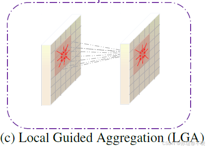
聚合范围相比于公式5 ：

调用顺序

python 复制代码

disp2 = self.disp2(x, g['lg1'], g['lg2'])  # torch.Size([1, 384, 1248])

python 复制代码

class DispAgg(nn.Module):

    def __init__(self, maxdisp=192):
        super(DispAgg, self).__init__()
        self.maxdisp = maxdisp
        self.LGA3 = LGA3(radius=2)
        self.LGA2 = LGA2(radius=2)
        self.LGA = LGA(radius=2)
        self.softmax = nn.Softmin(dim=1)
        self.disparity = DisparityRegression(maxdisp=self.maxdisp)
#        self.conv32x1 = BasicConv(32, 1, kernel_size=3)
        self.conv32x1=nn.Conv3d(32, 1, (3, 3, 3), (1, 1, 1), (1, 1, 1), bias=False)

    def lga(self, x, g):
        g = F.normalize(g, p=1, dim=1)  # torch.Size([1, 75, 384, 1248])
        x = self.LGA2(x, g)
        return x

    def forward(self, x, lg1, lg2):
        x = F.interpolate(self.conv32x1(x), [self.maxdisp+1, x.size()[3]*3, x.size()[4]*3], mode='trilinear', align_corners=False) # torch.Size([1, 32, 65, 128, 416])->torch.Size([1, 1, 193, 384, 1248])
        x = torch.squeeze(x, 1)  # torch.Size([1, 193, 384, 1248])
        assert(lg1.size() == lg2.size())
        x = self.lga(x, lg1)  # lg1:torch.Size([1, 193, 384, 1248])
        x = self.softmax(x)   # torch.Size([1, 193, 384, 1248])
        x = self.lga(x, lg2)  # torch.Size([1, 193, 384, 1248])
        x = F.normalize(x, p=1, dim=1)  # torch.Size([1, 193, 384, 1248])
        return self.disparity(x)

调用的时候有 softmax，不知道是不是对应该部分

-> lga 的 forward

python 复制代码

class Lga2Function(Function):   
    @staticmethod  
    def forward(ctx, input, filters, radius=1):
        ctx.radius = radius
        assert(input.is_contiguous() == True and filters.is_contiguous() == True)
        with torch.cuda.device_of(input):
            num, channels, height, width = input.size()  # torch.Size([1, 193, 384, 1248])
            temp_out = input.new().resize_(num, channels, height, width).zero_()
            output = input.new().resize_(num, channels, height, width).zero_()
            GANet.lga_cuda_forward(input, filters, temp_out, radius)
            GANet.lga_cuda_forward(temp_out, filters, output, radius)
            output = output.contiguous()  # torch.Size([1, 193, 384, 1248])
        ctx.save_for_backward(input, filters, temp_out)
        return output

cuda 代码

python 复制代码

void lga_forward (at::Tensor input, at::Tensor filters, at::Tensor output,
	     const int radius){

//        print_kernel<<<10, 10>>>();
//        cudaDeviceSynchronize();
  //       int num=input->size(0);
  int channel = input.size(1);
  int height = input.size(2);
  int width = input.size(3);
  int n = input.numel ();
  //       printf("%d, %d, %d, %d, %d\n", height, width, channel, n, radius);
  //       cudaStream_t stream = at::cuda::getCurrentCUDAStream();
/*        float *temp = new float[n];
        float *out = input.data<float>();
        cudaMemcpy(temp,out,n*sizeof(float),cudaMemcpyDeviceToHost);	
        for(int i=0;i<n;i++)
           printf("%.2f ", temp[i]);
*/
  lga_filtering_forward <<< (n + CUDA_NUM_THREADS - 1) / CUDA_NUM_THREADS,
    CUDA_NUM_THREADS >>> (n, input.data<float>(), filters.data<float>(),
			  height, width, channel, radius,
			  output.data<float>());
  //     temp = new float[n];


}

核心的 lga_filtering_forward 实现为

python 复制代码

// LGA（Local Guided Aggregation）前向 CUDA kernel
// 对代价体进行局部引导滤波：在 (2r+1)x(2r+1) 邻域内，对 d-1, d, d+1 视差平面加权聚合
__global__ void lga_filtering_forward(
    const int n,                // 总元素数 = B * D * H * W（通常 B=1）
    const float *bottom_data,   // 输入代价体指针，布局: [b][d][h][w]
    const float *filters,       // 引导权重指针，布局: [b][k][h][w][r][c]（k=3, r/c ∈ [-radius, radius]）
    const int height,           // 图像高度 H
    const int width,            // 图像宽度 W
    const int channel,          // 实际为视差级数 D（因视差被当作"通道"）
    const int radius,           // 滤波窗口半径（如 2 → 5x5 窗口）
    float *top_data             // 输出缓冲区，初始应为 0
) {
  // 计算当前线程处理的全局索引（每个线程负责一个输出元素）
  int index = blockIdx.x * blockDim.x + threadIdx.x;

  // 【调试】打印 OK（开发时使用）
  // printf("OK\n");
  // printf("%d, %.2f, %.2f\n", index, bottom_data[index], top_data[index]);

  // 边界检查：防止越界
  if (index >= n) {
    return;
  }

  // 【调试】强制设为 1.0（开发时使用）
  // top_data[index] = 1.0;
  // assert(0);

  // 每个视差平面（channel slice）的像素总数
  int step = height * width;  // = H * W

  // 滤波窗口边长（如 radius=2 → wsize=5）
  int wsize = 2 * radius + 1;

  // fbase: 当前线程在 filters 中的基地址（跳过 batch 维度）
  // filters 布局: [b][k][h][w][r][c] → 展平后:
  //   每个 batch 占: (3 * H * W * wsize * wsize) 个 float
  //   当前 batch 偏移: index / (step * channel) * (step * wsize * wsize * 3)
  //   加上空间位置偏移: index % step （即 h*W + w）
  int fbase = index / (step * channel) * (step * wsize * wsize * 3) + index % step;

  // 解码 index → (batch, depth, row, col)
  int row = index % step / width;   // 行号 h
  int col = index % width;          // 列号 w
  int depth = index / step % channel; // 视差索引 d

  // 初始化输出（注意：调用前需确保 top_data 已清零！）
  // 此处未显式初始化，依赖外部 memset 或 zero-filled tensor

  // 遍历三个视差偏移: d-1, d, d+1
  for (int d = -1; d <= 1; d++) {

    // 遍历空间邻域行偏移 [-radius, radius]
    for (int r = -radius; r <= radius; r++) {

      // 遍历空间邻域列偏移 [-radius, radius]
      for (int c = -radius; c <= radius; c++) {

        // 计算邻域中实际坐标
        int rr = r + row;   // 邻域行
        int cc = c + col;   // 邻域列
        int dd = d + depth; // 邻域视差

        // shift: 相对于当前 index 的偏移量（用于访问 bottom_data）
        // 若 (rr, cc, dd) 越界，则 shift=0（用自身代替，但实际应避免）
        int shift = 0;
        if (rr >= 0 && cc >= 0 && dd >= 0 && 
            rr < height && cc < width && dd < channel) {
          // 合法位置：shift = (dd - depth)*step + (rr - row)*width + (cc - col)
          // 但此处 dd = depth + d, rr = row + r, cc = col + c
          // 所以 shift = d*step + r*width + c
          shift = r * width + c + d * step;
        }
        // 注意：越界时 shift=0，会错误地累加 bottom_data[index]！
        // 更严谨的做法是跳过越界项（见后文说明）

        // location: 在 filters 中的局部偏移（对应 [k=d+1][r+radius][c+radius]）
        // k = d + 1 → {-1,0,1} 映射为 {0,1,2}
        // r + radius, c + radius → [0, wsize-1]
        int location = (d + 1) * (wsize * wsize) + (r + radius) * wsize + (c + radius);

        // 执行加权累加：
        //   top_data[index] += bottom_data[neighbor] * filter_weight
        top_data[index] += bottom_data[index + shift] * filters[fbase + location * step];
      }
    }
  }

  // 【调试】强制设为 1.0 并打印（开发时使用）
  // top_data[index] = 1.0;
  // printf("%d, %d, %d, %.2f, %.2f\n", index, row, col, bottom_data[index], top_data[index]);
}

（3）Efficient Implementation

SGA，guidance subnet is split, reshaped and normalized as four H x W x K x F (K =5) weight matrices for four directions' aggregation

LGA layer need to learn a H xW x 3 K 2 3K^2 3K2 xF (K = 5) weight

repeat the computation of EQ. (7) twice with the same weight matrix，也即 LGA 使用了两次

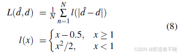
4.3、Loss Function

smooth L1

5、Experiments

240x576 random crops from the input images

max disparity 192

5.1、Datasets and Metrics

Scene Flow
KITTI 2012
KITTI 2015

Scene Flow dataset for 10 epochs，KITTI datasets fine-tune a further 640 epochs

评价指标

3-pixel threshold error rate
1-pixel threshold error rate
EPE

5.2、Ablation Study

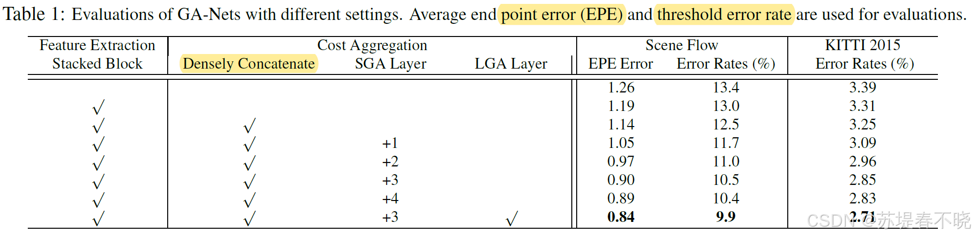
densely concatenate 是 feature extraction 模块当中的

5.3、Effects of Guided Aggregations

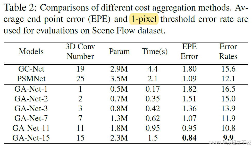
对比了 3D conv 的数量，作者方法 conv3D = 7 时效果就逼近 GC-Net 的19 和 PSMNet 的 25 了

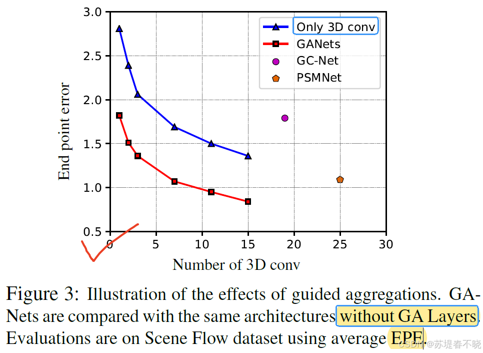
左下角效果最好，没有 GANet 的结构，效果下降明显

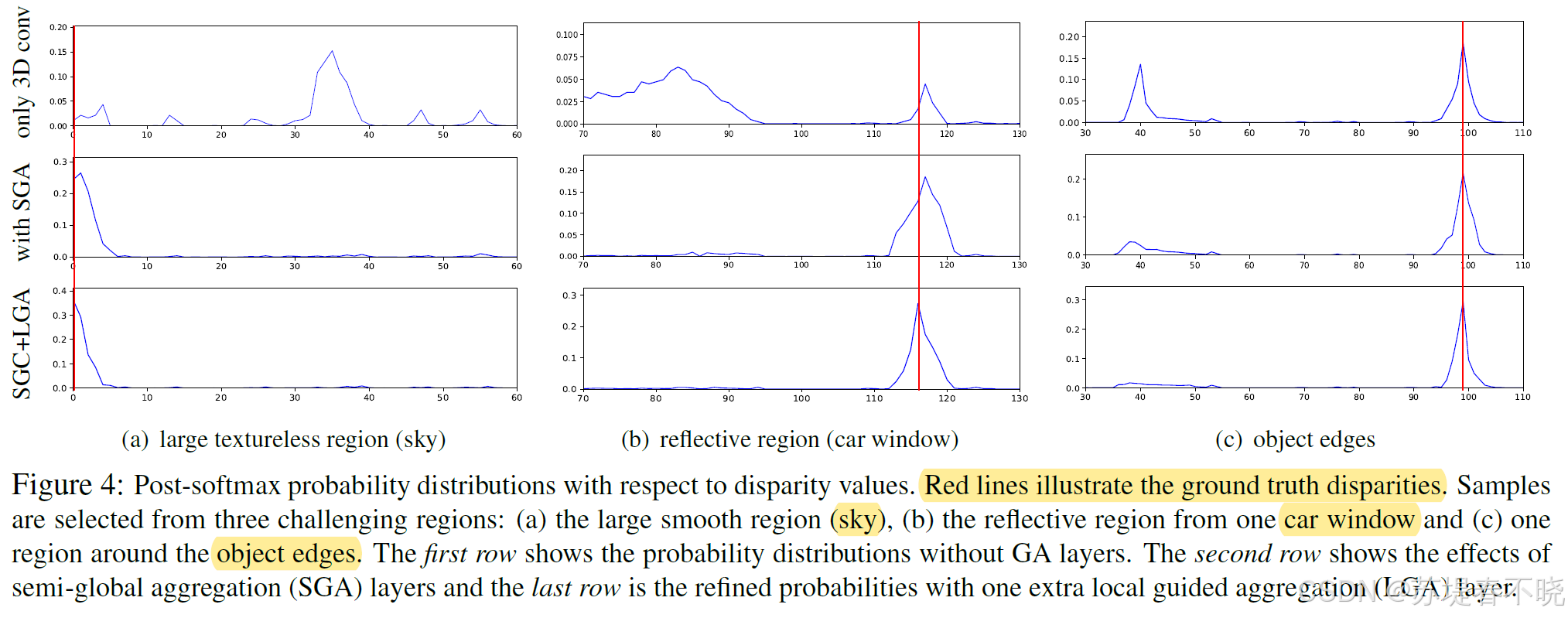
The SGA layers successfully suppress these noise in the probabilities by aggregating surrounding matching information

The LGA layer further concentrates the probability peak on the ground truth value.

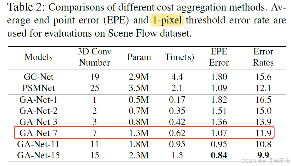
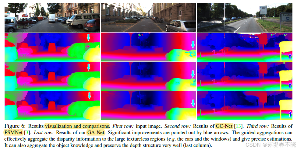
5.4、Comparisons with SGMs and 3D Convolutions

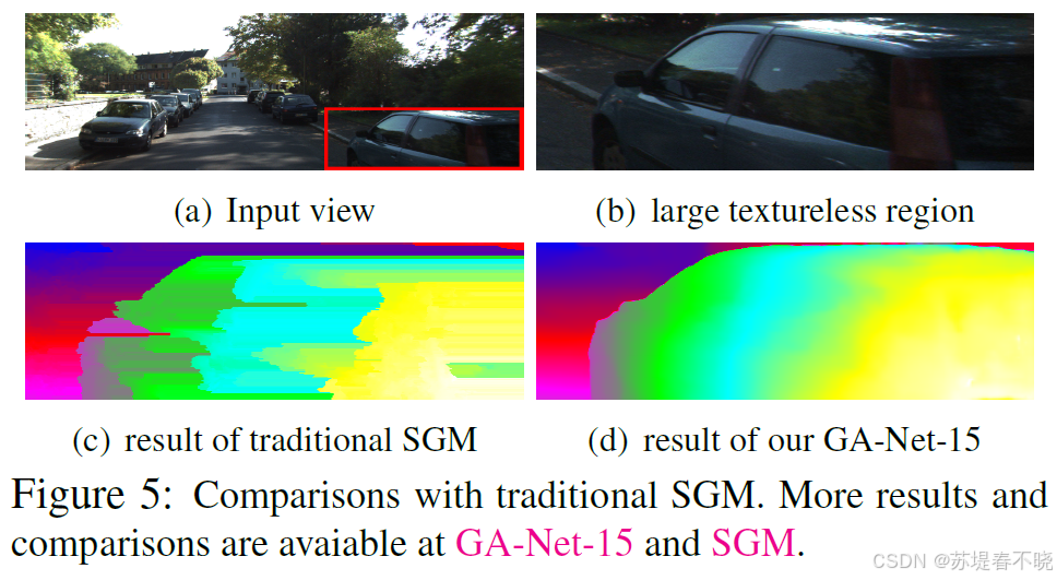
most of the fronto-parallel approximations in large textureless regions have been avoided.

The guidance subnet learns effective geometrical and contextual knowledge to control the directions, scopes and strengths of the cost aggregations

5.5、Complexity and Realtime Models

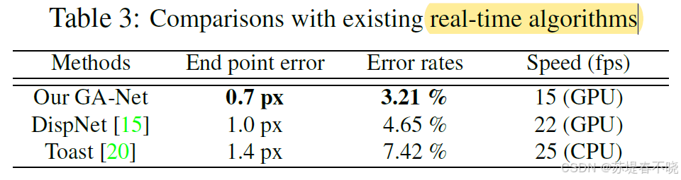
more efficient and effective than the 3D convolutional layer

3D conv 的计算复杂度， O ( K 3 C N ) O(K^3CN) O(K3CN)， N = H × W × D N = H×W×D N=H×W×D is the elements number of the output blob，C 是输入的 channel，K 是 conv 的 kernel

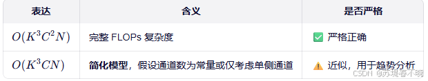
作者的 GANet 计算复杂度， O ( 4 K N ) O(4KN) O(4KN) or O ( 8 K N ) O(8KN) O(8KN) for 4 方向或者 8 方向 aggregation，K=5 是公式 5 中的 5 个 weights，

k = 3 k = 3 k=3，计算效率是 3D conv 的 100 倍

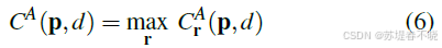
5.6、Evaluations on Benchmarks

Scene Flow Dataset

KITTI 2012 and 2015 Datasets

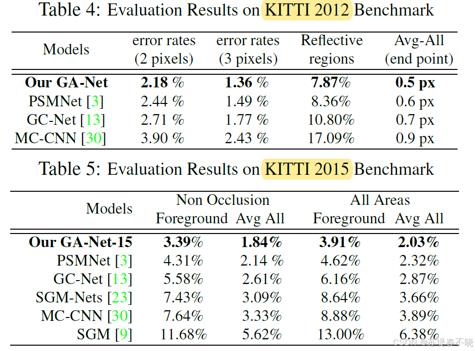
GA-Nets can effectively aggregate the correct matching information into the challenging large textureless or reflective regions to get precise estimations

6、Conclusion（own） / Future work

把传统方法 SGM 修改为可导的方式，融入到了网络中，增强 cost aggregation 模块的能力，替换 3D Conv 降低计算量
one GA layer 计算复杂度仅为 3D 卷积的 1/100（FLOPs）；
可端到端训练，无需手工调参；
在纹理缺失、反光、遮挡等挑战区域表现优异。
as occlusions,large textureless areas (e.g. sky, walls etc.), reflective surfaces(e.g. windows), thin structures and repetitive textures
The cost volume C is formed of matching costs at each pixel's location for each candidate disparity value d.
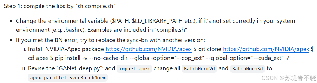
github 中注明了，作者自己的模块 GA、LA 是好编译 cuda 源码的，BN 不好编译，需要按照其介绍的借助 apex 修复替换方法
SGM，抑制不必要的跳变，但允许真实边缘存在。
hard-minimum selection leads to a lot of fronto parallel surfaces in depth estimations
cuda 源码需要再熟练熟练，编译成库之后好像不能单步调试
核心是公式 5 和公式 7
可以利用引导聚合层来代替3D convolution。（《GA-Net: Guided Aggregation Net for End-to-end Stereo Matching》）

更多论文解读，请参考【Paper Reading】

【GA-Net】《GA-Net: Guided Aggregation Net for End-to-end Stereo Matching》

文章目录

1、Background and Motivation

2、Related Work

3、Advantages / Contributions

4、Method

4.1、Network Architecture

4.2、Guided Aggregation Layers

4.3、Loss Function

5、Experiments

5.1、Datasets and Metrics

5.2、Ablation Study

5.3、Effects of Guided Aggregations

5.4、Comparisons with SGMs and 3D Convolutions

5.5、Complexity and Realtime Models

5.6、Evaluations on Benchmarks

6、Conclusion（own） / Future work