拆解指数加权平均:5 分钟看懂机器学习的 "数据平滑神器"
Ming | 2025.12

什么是指数加权平均?简单来说,它是一种用于将序列数据变得更加平滑的经典方法。在机器学习中,我们经常会遇到来自传感器、实验或训练过程的噪声数据,这些数据波动很大,不容易直接观察趋势。指数加权平均就像一个"数据平滑神器",能够有效过滤短期波动,突出长期趋势,帮助我们更好地理解数据变化。
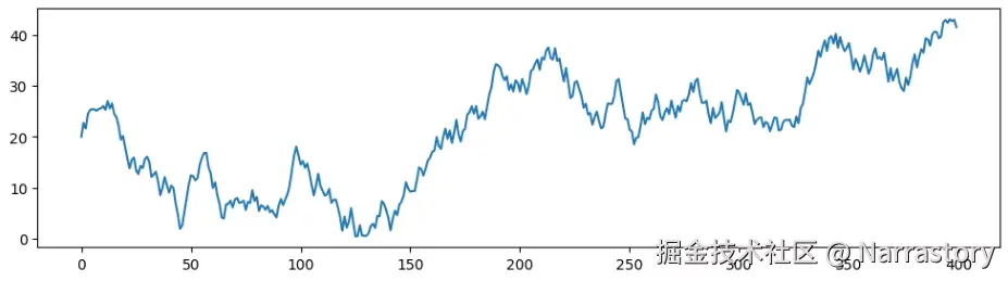
例如,下面是一个带有噪声的原始序列:
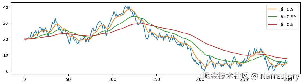
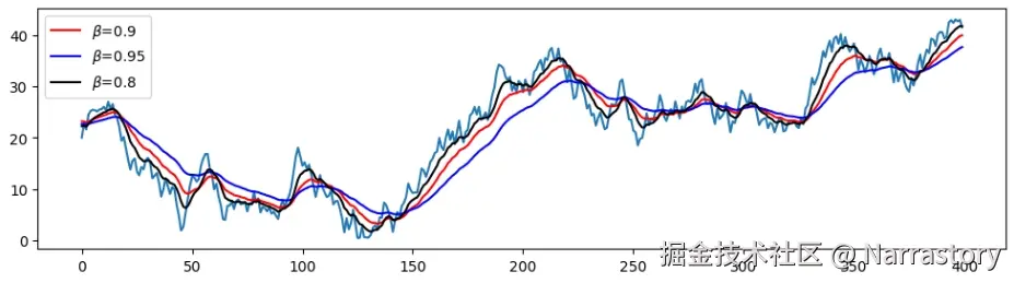
在使用不同平滑参数 β 的指数加权平均后,我们可以得到平滑程度各异的序列:
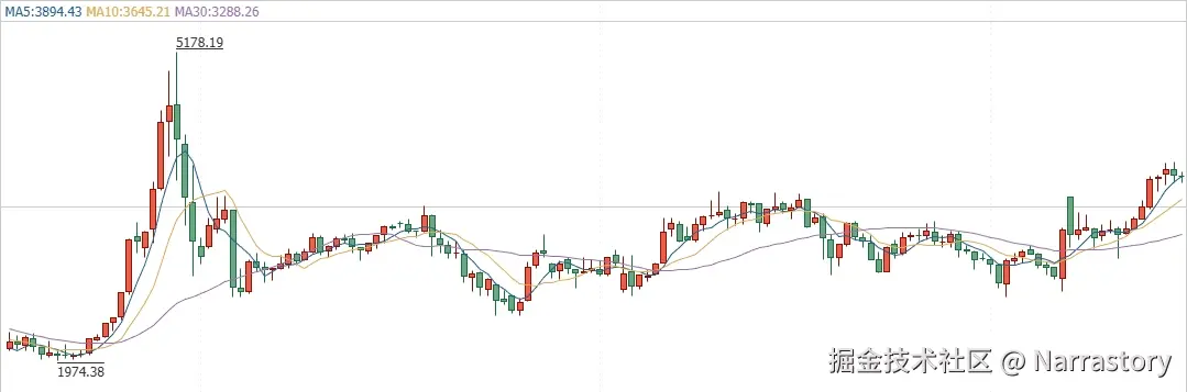
如果是了解过股票交易的朋友,应该对"移动平均线"(Moving Average)这个概念非常熟悉。它常被用于观察股价的趋势,帮助投资者过滤短期市场的"噪声",把握中长期的走势方向。其实,指数加权平均正是股票技术分析中"指数移动平均线"(Exponential Moving Average, EMA)的核心计算方法。
指数加权平均的实现非常简单,其本质是对历史数据进行加权组合,且权重随时间指数衰减。
假设我们有一个原始序列 a1,a2,...,an,我们希望得到一个平滑后的序列 b1,b2,...,bn。
通常我们令初始平滑值 b0=a0,然后从 n=1 开始迭代计算:
bn=βbn−1+(1−β)an
其中, β 是一个介于 0 和 1 之间的平滑因子。β 越大,曲线越平滑,但也会对最新数据的反应变得"迟钝";β 越小,平滑后的曲线越接近原始数据,保留的细节也越多。公式可以直观理解为:每一步的平滑值 bn 是上一时刻平滑值 bn−1 与当前观测值 an 的加权平均。
假设我们有一个长度为 5 的序列:
a=10,8,12,9,11
并取 β=0.8,初始值 b0=a0=10。我们一步步来计算 b1 到 b5:
- b1=0.8×10+0.2×8=8+1.6=9.6
- b2=0.8×9.6+0.2×12=7.68+2.4=10.08
- b3=0.8×10.08+0.2×9=8.064+1.8=9.864
- b4=0.8×9.864+0.2×11=7.8912+2.2=10.0912
最终平滑后的序列约为:
b=9.6,10.08,9.864,10.0912
可以看出,原本波动较大的 8,12,9,11 被平滑为一个变化更缓和的序列。
为什么这个公式能让一个曲线变得更加平滑呢?其实很好理解,从"惯性"的角度来看。当 β 很大(比如 0.9)时, bn−1 在更新中占据很大比重,当前的新值 an 只占很小的比例,这意味着平滑序列 b 具有强烈的"记忆"能力,不会因为某一点的突变而产生剧烈波动。反之,如果 β 很小(比如 0.1),则平滑序列会更紧密地跟踪原始数据的变化,适应更快,但平滑效果减弱。
不知道到这里你发现没有,上面的式子虽然能很好的平滑序列,但是有一个缺点,就是在序列刚开始的时候容易"失真"。从上面的展开式也可以看出,在序列开始时,我们令 b0=a0,由于历史数据较少, b0 的权重 β 较大,若 b0 与 a1,a2,... 差异明显,就会导致平滑序列初期出现"失真"。下面这张图就清晰展示了这个问题:
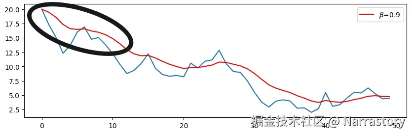
蓝色是原始曲线,红色是指数加权平均后的曲线。明显可见,红色曲线在开始阶段比蓝色高出不少,这是因为我们初始设置 b0=a0,而 a0 可能恰是一个较大或较小的异常值,影响了后续若干点的平滑结果。
那么如何解决这种失真呢,方法有很多,常用的解决方法之一是使用序列前若干点的平均值作为初始值 ,而不是直接使用 a0。
具体做法是:
- 选取一个合适的初始窗口长度 k(例如 k=5 或 k=10,根据序列总体长度和噪声情况决定)。
- 计算前 k 个原始数据的平均值: b0=k1∑i=1kai
这样做的优点是能够抵消个别异常点对平滑初期的影响,使平滑曲线从一开始就更贴合数据的整体趋势。一般来说, k 不宜过大,否则会引入不必要的滞后;如果数据在开始阶段变化剧烈,也可适当缩小 k,让平滑过程更快适应当前趋势。

接下来,我们用Python来实际操作演示一下指数加权平均的效果。这个例子会用到NumPy和Matplotlib库,我们将一步步生成带噪声的序列,并用不同参数进行平滑处理。
首先,引入必要的库,并定义一个用于生成平滑随机序列的辅助类SmoothRandomSequence
python
import numpy as np
import matplotlib.pyplot as plt
import random

class SmoothRandomSequence:
    def __init__(self, low, high, initial_value=None, max_step=None):
        self.low = low
        self.high = high
        self.range_width = high - low
        if initial_value is None:
            self.current = random.uniform(low, high)
        else:
            self.current = min(high, max(low, initial_value))
        if max_step is None:
            self.max_step = self.range_width * 0.1
        else:
            self.max_step = max_step
    def next(self):
        step = random.uniform(-self.max_step, self.max_step)
        next_value = self.current + step
        if next_value < self.low:
            next_value = self.low + (self.low - next_value)
        elif next_value > self.high:
            next_value = self.high - (next_value - self.high)
        next_value = max(self.low, min(self.high, next_value))
        self.current = next_value
        return next_value
    def generate_sequence(self, n):
        sequence = [self.current]
        for _ in range(n - 1):
            sequence.append(self.next())
return sequence这个SmoothRandomSequence类的具体实现细节不重要,你只需要知道它能生成一个在指定范围内波动、变化相对平滑的随机序列,模拟真实场景中带有噪声的数据。
现在,让我们使用这个类来生成一个包含300个数据点的原始序列:
python
# 创建平滑随机数生成器实例
# 设置范围0到60,初始值20,最大步长3
generator = SmoothRandomSequence(low=0, high=60, initial_value=20, max_step=3)

# 生成300个随机数的原始序列
noise_array = np.array(generator.generate_sequence(300))

# 绘图
fig, ax = plt.subplots(figsize=(10, 3))
ax.plot(noise_array)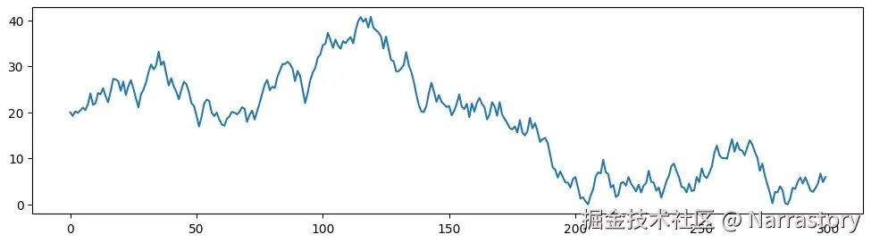
然后写一个名为exponential_weighted_average的函数,这个函数需要传入一个原始numpy序列,beta值和初始窗口大小 k就可以返回平滑后的序列,返回的序列类型也是numpy序列
python
def exponential_weighted_average(sequence, beta, initial_window=None):
    """
    参数:
    sequence: numpy数组,原始序列
    beta: 平滑因子,取值范围0~1
    initial_window: 用于计算初始平均值的窗口大小

    返回:
    平滑后的序列,长度与原始序列相同
    """
    n = len(sequence)
    smoothed = np.zeros(n)

    # 计算初始值
    if initial_window is not None and initial_window > 0:
        k = min(initial_window, n)
        smoothed[0] = np.mean(sequence[:k])
    else:
        smoothed[0] = sequence[0]

    # 迭代计算指数加权平均
    for i in range(1, n):
        smoothed[i] = beta * smoothed[i - 1] + (1 - beta) * sequence[i]

return smoothed最后,我们使用上面定义的exponential_weighted_average函数,来计算并且绘制三种不同 β下的平滑后的曲线
python
fig, ax = plt.subplots(figsize=(12, 3))

# 计算三种不同beta下的平滑结果
array1 = exponential_weighted_average(noise_array,beta = 0.95,initial_window=4)
array2 = exponential_weighted_average(noise_array,beta = 0.9,initial_window=4)
array3 = exponential_weighted_average(noise_array,beta = 0.8,initial_window=4)

# 绘制
ax.plot(noise_array)
ax.plot(array1, label=r"$\beta$=0.95")
ax.plot(array2, label=r"$\beta$=0.9")
ax.plot(array3, label=r"$\beta$=0.8")
ax.legend()