1.自定义模型进行手写数字的识别例子
2.直接用预训练模型识别图像
3.迁移学习
4.风格迁移
1. 识别手写数字 MNIST(自定义)
输入图像(28×28×1) → 卷积(32个3×3核) → 26×26×32
↓
卷积(64个3×3核) → 24×24×64
↓
最大池化(2×2) → 12×12×64
↓
Dropout(0.25) → 随机丢弃25%连接
↓
Flatten → 展平为9,216维向量
↓
全连接(128个神经元) → 128维向量
↓
Dropout(0.5) → 随机丢弃50%连接
↓
全连接(10个神经元) → 10维概率向量
↓
输出:数字0-9的概率分布
1.1****导入并查看数据集
从keras的自带数据集中导入所需的MNIST from import
加载数据到keras mnist.load_data()
可查看数据集的形状 shape
打印索引0对应训练集和测试集的图片
from matplotlib import pyplot plt.imshow(x_train0)
下载对应的库,可用pip或者conda下载最新版本,如果有gpu可下载gpu版本的,具体的命令直接把代码复制后,问ai就行。
1.2 数据预处理
01****处理灰度图片RAG彩色图片有3个通道,图片深度depth为3,灰度深度为1
后台程序为TensorFlow(n,width,height,depth) x_train.reshape(6000,28,28,1)
后台程序为Theano(n.depth,width,height) x_ train.reshape(6000,1,28,28)
使用函数image_data_format()=='channels_first'获取通道位置,if else判断即可
02数据转换为【0**,****1】**范围
X_train = x train.astype('float32')
x_test = x test.astype('float32')
原始图像数据通常是uint8(0-255的整数),神经网络需要浮点数进行计算,float32比float64占用更少内存,计算更快,精度通常足够;
X_train /= 254
x_test /= 255
归一化(Normalization),将像素值从0, 255范围缩放到0, 1,因为梯度下降在归一化数据上收敛更快,可以避免数值过大或过小,防止梯度消失/爆炸,确保像素值在相近范围,不同样本的尺度一致,提高模型稳定性。
归一化和数据转换还有很多其他的方式,主要是根据需求来选择。
03 数据标签预处理
查看数据标签 shape ; 将标签数据转换为二值数据格式
y_train = keras.utils.to_categorical(y _train, 10)
y_test = keras.utils.to_categorical(y _test, 10)
独热编码(one-hot):将分类标签(10个类别)转换为二进制向量的方法,只有一个元素是1,其余都是0,没有保留语义;
换成词嵌入可以保留数据的语义;
1.3****定义模型结构
神经层层数,每一层神经元数量和神经元连接方式
序贯模型逐层构建神经网络
Import sequential
sequential 线性堆叠层的简单模型,适用于单输入单输出的简单神经网络结构
model= sequential() 初始化
第一层二维卷积层
Model.add(Conv2D(32,kernel_size=(3,3),activation='relu',input_shape=(28,28,1)))
Conv2D:二维卷积层,用于提取图像特征
32:卷积核数量(输出通道数)
kernel_size=(3, 3):3×3的卷积核大小
activation='relu':ReLU激活函数(f(x)=max(0,x))
input_shape=(28, 28, 1):输入形状(高28,宽28,通道数1(灰度图))
计算过程:
输入:28×28×1的灰度图像,使用32个3×3卷积核扫描图像
输出:26×26×32的特征图(28-3+1=26)
参数量:(3×3×1+1)×32 = 320个参数
3×3:卷积核大小 ×1:输入通道数(灰度图) +1:每个滤波器有一个偏置项 ×32:32个滤波器
第二层二维卷积层
model.add(Conv2D(64, (3, 3), activation='relu'))
输入:26×26×32的特征图,使用64个3×3卷积核
输出:24×24×64的特征图(26-3+1=24)
参数量:(3×3×32+1)×64 = 18,496个参数
池化层:降低特征图尺寸,保留主要特征,防止过拟合
model.add(MaxPooling2D(pool_size=(2, 2)))
默认步长=池化窗口大小(不重叠池化)
2×2的池化窗口,每个2×2区域取最大值
输出形状:(24,24,64) → (12,12,64)
参数量:0(只有固定操作,无学习参数)
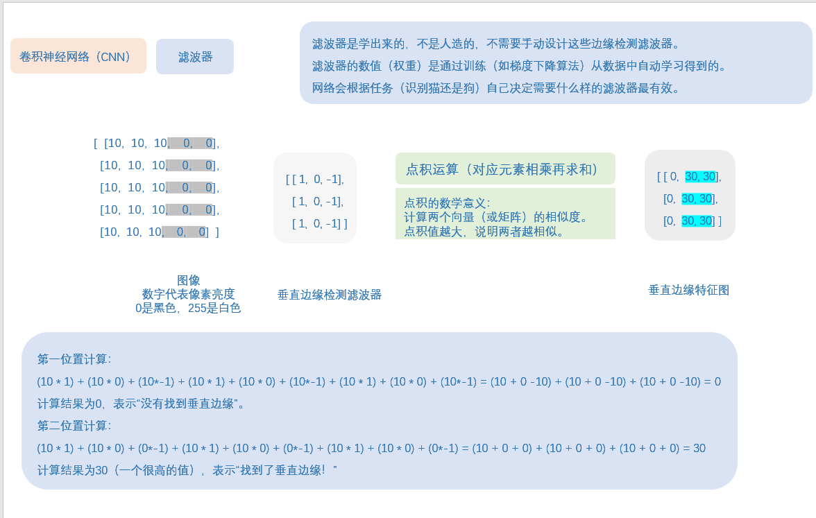
这里有一个概念叫:滤波器,去了解一下,就知道神经网络,权重,特征图,这些是什么东西了。
这里给点笔记,不用看懂,因为我写的,应该只有我自己懂,这里就是给个参考,你们自己去了解清楚,也搞一个笔记梳理一下。
第一个Dropout层:
model.add(Dropout(0.25))
随机丢弃25%的神经元连接,就是25%的输入单元被随机设为0,防止过拟合。
Flatten 层:将多维张量展平为一维向量
model.add(Flatten())
计算过程:
输入:12×12×64 = 9,216维的张量
输出:9,216维的一维向量
参数量:0(只有固定操作,无学习参数)
Dense:全连接层(密集层)
model.add(Dense(128, activation='relu'))
activation='relu':ReLU激活函数
计算过程:
输入:9,216维向量
输出:128维向量
参数量:9,216×128 + 128 = 1,179,776个参数
128:每个输入神经元连接到128个输出神经元,+ 128:偏置项
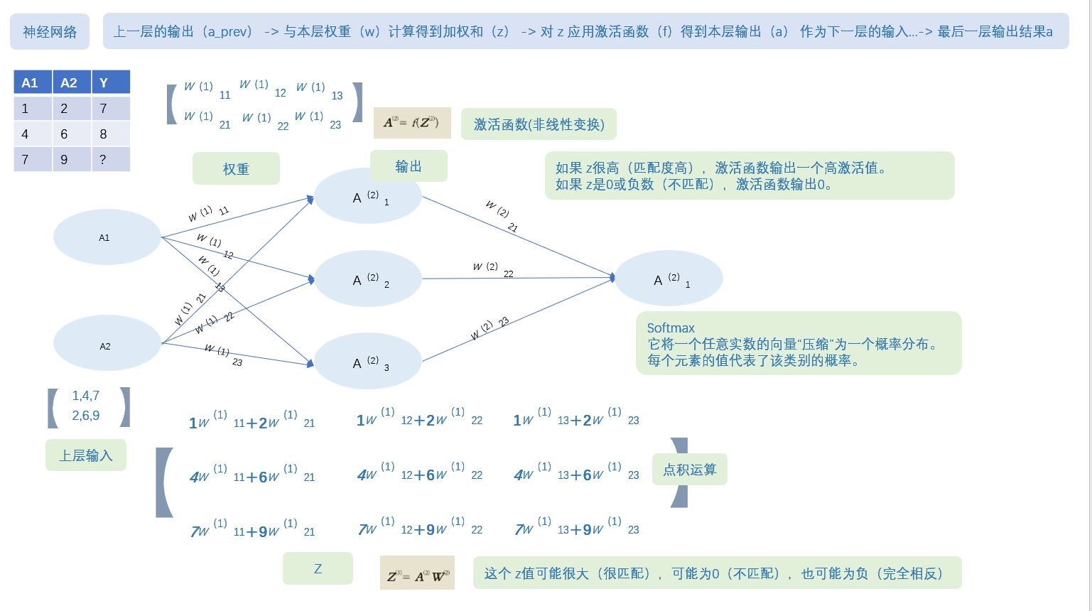
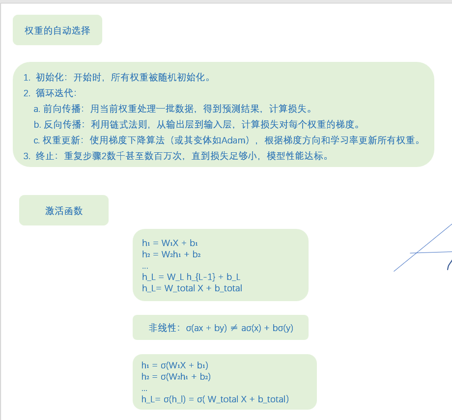
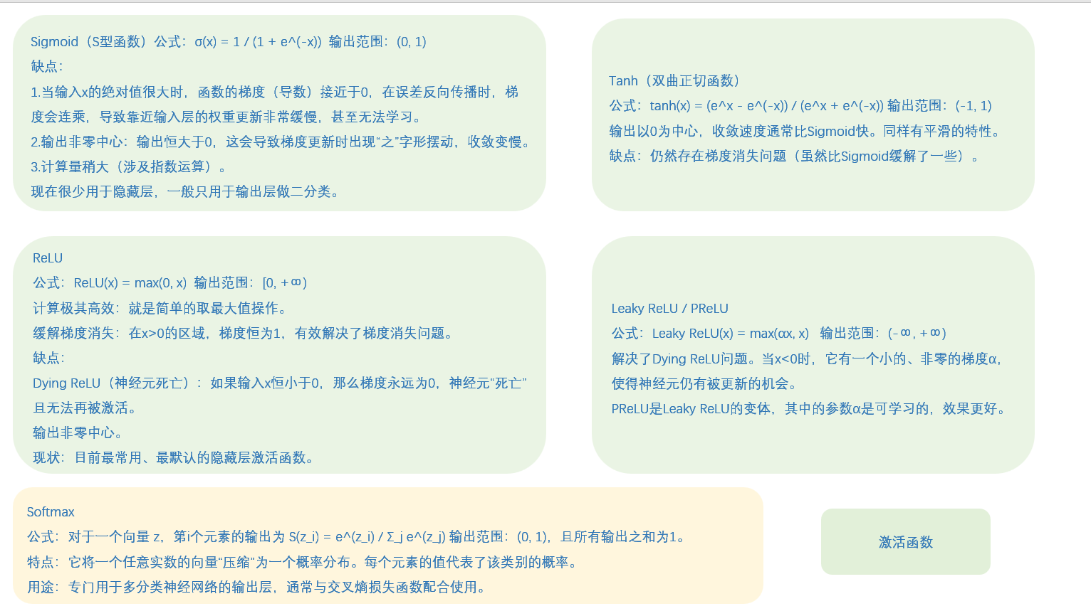
激活函数------很重要,是神经网络的关键,就是在简单的加权求和外面套一个函数,把整个过程从线性变成非线性了。
这里放一点笔记,稍微看一下,不用看懂,自己去了解清楚:
第二个Dropout层:
model.add(Dropout(0.5))
丢弃率50%,更高因为全连接层参数多易过拟合
输出层:输出10个类别的概率分类
model.add(Dense(10, activation='softmax'))
10:对应10个数字类别(0-9)
activation='softmax':将输出转换为概率分布
计算过程:
输入:128维向量
输出:10维概率向量(总和为1)
参数量:128×10 + 10 = 1,290个参数
完整运行代码:
python
# -*- coding: utf-8 -*-
import keras
from keras.datasets import mnist
from keras.models import Sequential
from keras.layers import Dense, Dropout, Flatten
from keras.layers import Conv2D, MaxPooling2D
from keras import backend as K

# 类别数量,它决定了输出层的神经元数量
num_classes = 10
# 批次大小
batch_size = 128
# 训练轮数
epochs = 12
# 确定输入图像的维度
img_rows, img_cols = 28, 28

# 使用load_data,在导入数据时可以把测试集与训练集直接分开
(x_train, y_train), (x_test, y_test) = mnist.load_data()

# 使用backend后台的K.image_data_format()获取通道在通道中的位置是一个不错的选择
if K.image_data_format() == 'channels_first':
    x_train = x_train.reshape(x_train.shape[0], 1, img_rows, img_cols)
    x_test = x_test.reshape(x_test.shape[0], 1, img_rows, img_cols)
    input_shape = (1, img_rows, img_cols)
else:
    x_train = x_train.reshape(x_train.shape[0], img_rows, img_cols, 1)
    x_test = x_test.reshape(x_test.shape[0], img_rows, img_cols, 1)
    input_shape = (img_rows, img_cols, 1)

# 数据类型转换
x_train = x_train.astype('float32')
x_test = x_test.astype('float32')
x_train /= 255
x_test /= 255

# 打印形状
print('x_train shape:', x_train.shape)
print(x_train.shape[0], 'train samples')
print(x_test.shape[0], 'test samples')

# 把一维的类别向量转化成二值向量形式
y_train = keras.utils.to_categorical(y_train, num_classes)
y_test = keras.utils.to_categorical(y_test, num_classes)

# 初始化模型
model = Sequential()
# 逐层添加神经层
model.add(Conv2D(32, kernel_size=(3, 3), activation='relu', input_shape=input_shape))
model.add(Conv2D(64, (3, 3), activation='relu'))
model.add(MaxPooling2D(pool_size=(2, 2)))
model.add(Dropout(0.25))
model.add(Flatten())
model.add(Dense(128, activation='relu'))
model.add(Dropout(0.5))
model.add(Dense(num_classes, activation='softmax'))

# 模型编译,定义了交叉熵损失、优化器和精度指标
model.compile(loss=keras.losses.categorical_crossentropy,
              optimizer=keras.optimizers.Adadelta(),
              metrics=['accuracy'])

# 开始训练,并保存训练历史记录到变量`history`中
history = model.fit(x_train, y_train,
                    batch_size=batch_size,
                    epochs=epochs,
                    verbose=1,
                    validation_data=(x_test, y_test))

# 模型评估
score = model.evaluate(x_test, y_test, verbose=0)
print('Test loss:', score[0])
print('Test accuracy:', score[1])

# 使用Matplotlib简单可视化
import matplotlib.pyplot as plt
# 列出history中的所有关键字
print(history.history.keys())
# 显示accuracy
plt.plot(history.history['acc'])
plt.plot(history.history['val_acc'])
plt.title('model accuracy')
plt.ylabel('accuracy')
plt.xlabel('epoch')
plt.legend(['train', 'test'], loc='upper left')
plt.show()
# 显示loss
plt.plot(history.history['loss'])
plt.plot(history.history['val_loss'])
plt.title('model loss')
plt.ylabel('loss')
plt.xlabel('epoch')
plt.legend(['train', 'test'], loc='upper left')
plt.show()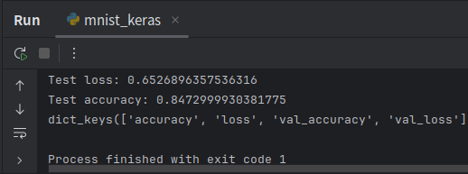
2.直接用预训练模型识别图像
不推荐你们直接运行代码,因为VGG16有528 MB,可以替换为ResNet50只有98M,或者不用运行看一下得了,没什么差别的。
python
from keras.applications.vgg16 import VGG16
from keras.preprocessing import image
from keras.applications.vgg16 import preprocess_input, decode_predictions
import numpy as np
import os
import matplotlib.pyplot as plt

# 初始化模型
model = VGG16(weights='imagenet', include_top=True)
# VGG16: 预训练的卷积神经网络模型
# weights='imagenet': 使用ImageNet数据集预训练的权重
# include_top=True: 包含顶层的全连接层 如果为false就涉及迁移学习

# 查看模型结构

model.summary()  # summary: 打印模型的结构摘要,显示各层信息和参数数量

# 导入图像
# 在此处填写自己的图片路径
img_path = "./test/cat.jpg"
img = image.load_img(img_path, target_size=(224, 224))
# img: 加载的图像对象
# load_img: 加载图片的函数
# target_size=(224, 224): 指定图片调整为224x224像素

# 显示图像
plt.imshow(img)  # imshow: 显示图片
plt.axis('off')  # 关闭坐标轴显示
plt.show()  # show: 显示图形窗口

# 预处理
x = image.img_to_array(img)
# img_to_array: 将图片转换为numpy数组的函数

x = np.expand_dims(x, axis=0)
# expand_dims: 扩展数组维度的函数
# axis=0: 在第0维(最外层)增加维度
# 从(224, 224, 3)变为(1, 224, 224, 3)

# 预处理vgg16适合的输入形式
x = preprocess_input(x)  # preprocess_input: VGG16专用的图片预处理函数

# 对预处理后的图片数据进行预测
features = model.predict(x)
# predict: 进行预测的函数

predictions = decode_predictions(features, top=3)[0]
# decode_predictions: 解码预测结果的函数(把预测结果翻译成容易读懂的(class, description, probability)形式)
# top=3: 只显示前3个最可能的结果  [0]: 取列表的第一个元素(批次中的第一张图片)

print('预测结果:')
for i, (imagenet_id, label, prob) in enumerate(predictions):
    print(f'{i+1}. {label}: {prob:.2%}')
# enumerate: 同时获取索引和元素的函数
# f-string: 格式化字符串 {i+1}: 排名(从1开始){label}: 类别名称 {prob:.2%}: 概率值,以百分比显示,保留2位小数

print(f'\n模型识别为: {predictions[0][1]} (置信度: {predictions[0][2]:.2%})')
# predictions[0]: 第一个预测结果 [1]: 元组的第二个元素(类别名称) [2]: 元组的第三个元素(概率值)
# {predictions[0][1]}: 最可能类别的名称
# {predictions[0][2]:.2%}: 最可能类别的概率值
3.迁移学习
迁移学习包含两种核心方法:
01 特征提取器法:冻结预训练模型的所有卷积层权重,移除原分类层,仅训练新添加的任务特定层。这种方法适用于数据较少、任务相似的情况,能快速实现迁移且成本低。
02 微调法:以较小学习率解冻并更新部分或全部卷积层权重,同时训练新分类层。这种方法适用于数据充足、任务差异较大的情况,能实现更精准的领域适应,但需要更多计算资源。
实践中常先进行特征提取训练,再进行局部微调,平衡效率与精度。
python
本例中使用的这个数据集可以在Kaggle的官方网站(https://www.kaggle.com/tongpython/cat-and-dog)下载。首先要加载预训练的VGG16,这里使用include_top=False,即不包含顶部的连接层。

# -*- coding: utf-8 -*-

from keras import applications
from keras.preprocessing.image import ImageDataGenerator
from keras import optimizers
from keras.models import Model
from keras.layers import Flatten, Dense
from keras.callbacks import ModelCheckpoint, EarlyStopping
import matplotlib.pyplot as plt

# 设置图像尺寸
img_width, img_height = 224, 224

# 设置数据目录路径
train_data_dir = './data/dog_cat/training_set'  # 训练集目录
validation_data_dir = './data/dog_cat/test_set'  # 验证集目录

# 设置训练参数
batch_size = 100  # 批次大小
epochs = 50  # 训练轮数

# 模型加载
# 加载VGG16预训练模型,不包含顶层全连接层
model = applications.VGG16(weights="imagenet", include_top=False,
                          input_shape=(img_width, img_height, 3))

# 冻结部分卷积层(前11层),这些层提取一般特征,设置为不可训练
for layer in model.layers[0:11]:
    layer.trainable = False

# 添加自定义的网络结构
x = model.output  # 获取VGG16卷积部分的输出
x = Flatten()(x)  # 将多维特征展平为一维
x = Dense(4096, activation="relu")(x)  # 全连接层,4096个神经元
x = Dense(1024, activation="relu")(x)  # 全连接层,1024个神经元
predictions = Dense(2, activation="softmax")(x)  # 输出层,2个神经元(猫狗二分类)

# 完成模型构建
model_final = Model(inputs=model.input, outputs=predictions)

# 模型编译
model_final.compile(
    loss="categorical_crossentropy",  # 分类交叉熵损失函数
    optimizer=optimizers.SGD(lr=0.0001, momentum=0.9),  # SGD优化器
    metrics=["accuracy"]  # 评估指标为准确率
)

# 使用数据增广初始化训练数据生成器
train_datagen = ImageDataGenerator(
    rescale=1./255,  # 像素值归一化到0-1范围
    horizontal_flip=True,  # 水平翻转
    fill_mode="nearest",  # 填充模式
    zoom_range=0.3,  # 随机缩放范围
    width_shift_range=0.3,  # 水平平移范围
    height_shift_range=0.3,  # 垂直平移范围
    rotation_range=30  # 随机旋转角度
)

# 验证集数据生成器(通常不需要做过多增强)
test_datagen = ImageDataGenerator(
    rescale=1./255,  # 只做归一化
    horizontal_flip=True,
    fill_mode="nearest",
    zoom_range=0.3,
    width_shift_range=0.3,
    height_shift_range=0.3,
    rotation_range=30
)

# 训练数据生成器
train_generator = train_datagen.flow_from_directory(
    train_data_dir,  # 训练集目录
    target_size=(img_height, img_width),  # 调整图像大小
    batch_size=batch_size,  # 批次大小
    class_mode="categorical",  # 分类模式
    seed=999  # 随机种子
)

# 验证数据生成器
validation_generator = test_datagen.flow_from_directory(
    validation_data_dir,  # 验证集目录
    target_size=(img_height, img_width),  # 调整图像大小
    batch_size=batch_size,  # 批次大小
    class_mode="categorical",  # 分类模式
    seed=999  # 随机种子
)

# 设定训练终止条件
# 模型检查点回调,保存最佳模型
checkpoint = ModelCheckpoint(
    "vgg16_dog_cat_only_full_connect.h5",  # 保存的文件名
    monitor='val_accuracy',  # 监控验证集准确率
    verbose=1,  # 显示详细信息
    save_best_only=True,  # 只保存最佳模型
    save_weights_only=False,  # 保存整个模型
    mode='auto',  # 自动选择模式
    save_freq='epoch'  # 每个epoch保存一次
)

# 早停回调,防止过拟合
early = EarlyStopping(
    monitor='val_accuracy',  # 监控验证集准确率
    min_delta=0,  # 最小变化阈值
    patience=10,  # 耐心值
    verbose=1,  # 显示详细信息
    mode='auto'  # 自动选择模式
)

# 模型训练
print("开始训练模型...")
fit_history = model_final.fit(
    train_generator,
    steps_per_epoch=len(train_generator),  # 每个epoch的步数
    epochs=epochs,  # 训练轮数
    validation_data=validation_generator,  # 验证数据
    validation_steps=len(validation_generator),  # 验证步数
    callbacks=[checkpoint, early]  # 回调函数
)

print("模型训练完成!")

# 可视化训练结果
plt.figure(1, figsize=(15, 8))

# 子图1:准确率曲线
plt.subplot(221)
plt.plot(fit_history.history['accuracy'])
plt.plot(fit_history.history['val_accuracy'])
plt.title('Model Accuracy')
plt.ylabel('Accuracy')
plt.xlabel('Epoch')
plt.legend(['Train', 'Validation'], loc='upper left')

# 子图2:损失曲线
plt.subplot(222)
plt.plot(fit_history.history['loss'])
plt.plot(fit_history.history['val_loss'])
plt.title('Model Loss')
plt.ylabel('Loss')
plt.xlabel('Epoch')
plt.legend(['Train', 'Validation'], loc='upper left')

plt.tight_layout()  # 自动调整子图参数
plt.show()

# 打印训练摘要
print(f"训练集准确率: {max(fit_history.history['accuracy']):.4f}")
print(f"验证集准确率: {max(fit_history.history['val_accuracy']):.4f}")
print(f"最终训练集损失: {fit_history.history['loss'][-1]:.4f}")
print(f"最终验证集损失: {fit_history.history['val_loss'][-1]:.4f}")

# 保存最终模型
model_final.save("final_dog_cat_classifier.h5")
print("模型已保存为 'final_dog_cat_classifier.h5'")
4.风格迁移
想象一下你向别人描述一幅画:
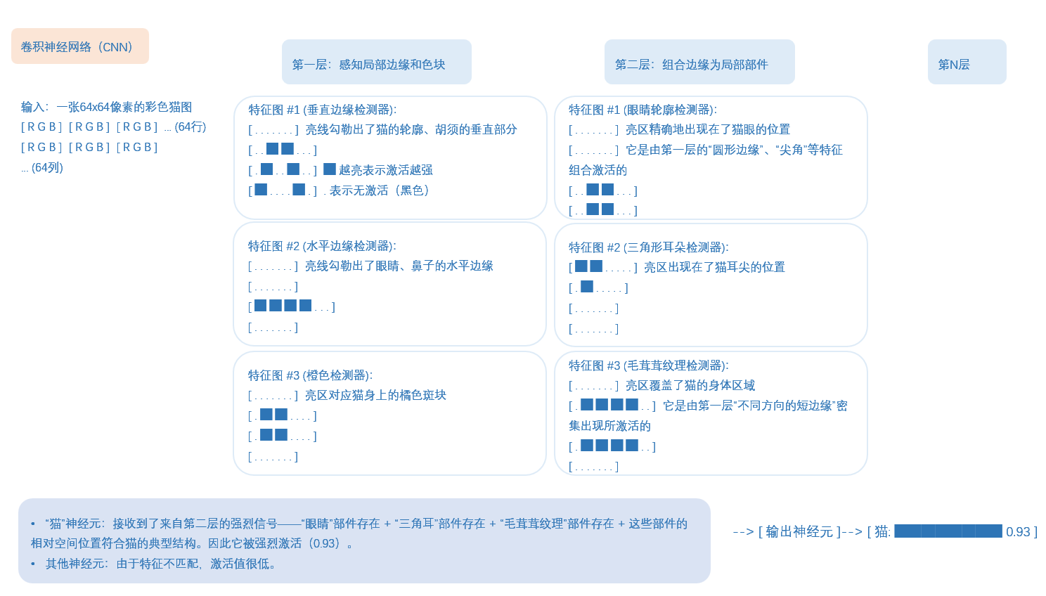
浅层特征(像眼睛看到的原始画面):这里有红色,那里有蓝色这里有直线,那里有曲线
深层特征(像理解画面含义):"这是一只猫坐在沙发上""这是一栋房子前面有棵树"
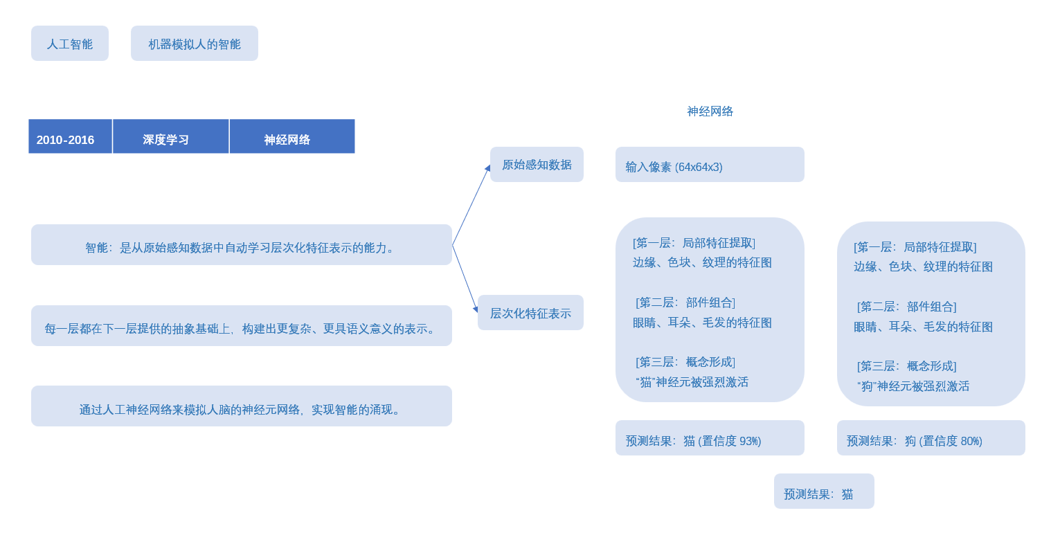
风格迁移的目标是生成一张新图像,不断迭代,使其同时具备内容图像的深层语义内容(物体、结构、布局)和风格图像的浅层特征(笔触、纹理、色彩分布等表现手法)。
将风格迁移问题转化为优化问题:
总损失 = α × 内容损失 + β × 风格损失
其中:
α, β 是超参数,控制内容与风格的相对权重
通过优化生成图像的像素值来最小化总损失
使用预训练的CNN(如VGG19)作为特征提取器,网络参数固定
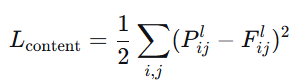
4.1 内容损失 (Content Loss)
P:内容图像在VGG网络第L层的特征图(目标)F:生成图像在同一层(L层)的特征图(当前结果)
i,j:遍历所有位置(第几个像素)和所有通道(第几个特征)
平方差:计算损失("它们有多像",损失越小越相似)
通常VGG16里,选择conv4_2(物体的基本形状)或者 conv5_2(物体类别、抽象概念)
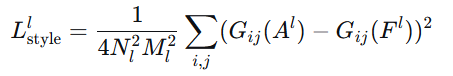
4.2 风格损失 (Style Loss)
Gram矩阵就是记录:
当你用1号笔时,是否经常同时用3号笔?
当你用2号笔时,是否经常同时用4号笔?
这些笔的"搭档关系"就是绘画风格。
算法讲解:
第一步:提取特征
原始特征图:高×宽×通道 H, W, C
例如:14×14×512(高14像素,宽14像素,512个通道)
reshape成:196, 512 (HW相乘:14×14=196,C:512个通道)
现在每行是一个像素,每列是一个特征通道
第二步:计算相关性
特征矩阵
F = \[1, 0, 2, # 像素1:通道1=1,通道2=0,通道3=2
0, 1, 1, # 像素2
2, 1, 0] # 像素3
Gram矩阵 = F转置 × F
G1,1 = 1×1 + 0×0 + 2×2 = 5 (通道1的自相关)
G1,2 = 1×0 + 0×1 + 2×1 = 2 (通道1和通道2的相关性)
以此类推...
G1,2=2 表示:在这张图片中,当特征1出现时,特征2也倾向于出现
这些"特征搭档关系"就定义了风格
单层:
多层:
内容:只需要保持主要结构,一层即可
风格:需要从细节到整体全面模仿,需要多层
伪代码描述
加载预训练VGG19,冻结所有参数
定义内容层和风格层集合
提取内容图像在内容层的特征图作为内容目标
提取风格图像在风格层的特征图,计算Gram矩阵作为风格目标
初始化生成图像(常用:内容图像副本 + 噪声)
For iteration = 1 to max_iterations:
a. 前向传播生成图像通过VGG网络
b. 计算内容损失:生成图像内容层特征 vs 内容目标
c. 计算风格损失:各风格层Gram矩阵 vs 风格目标
d. 计算总损失 = α×内容损失 + β×风格损失
e. 反向传播计算梯度(只对生成图像)
f. 更新生成图像像素值
- 返回优化后的生成图像

python
# -*- coding: utf-8 -*-

from __future__ import print_function
from keras.preprocessing.image import load_img, save_img, img_to_array
import numpy as np
from scipy.optimize import fmin_l_bfgs_b
import time
import warnings

from keras.applications import vgg19
from keras import backend as K

warnings.filterwarnings('ignore')

# 设置图像路径
base_image_path = "./data/content.jpg"  # 内容图像路径
style_reference_image_path = "./data/starry_night.jpg"  # 风格图像路径
result_prefix = 'result_'  # 结果图像前缀

# 设置损失函数权重
total_variation_weight = 1.0  # 总变差损失权重
style_weight = 1.0  # 风格损失权重
content_weight = 0.025  # 内容损失权重

# 设置迭代次数
iterations = 10

# 获取内容图像的尺寸,并设置生成图像的大小
width, height = load_img(base_image_path).size
img_nrows = 400  # 设置图像高度为400像素
img_ncols = int(width * img_nrows / height)  # 按比例计算宽度

# 预处理函数:将图像转换为VGG19模型所需的格式
def preprocess_image(image_path):
    """
    加载图像并进行预处理,使其符合VGG19模型的输入要求
    """
    img = load_img(image_path, target_size=(img_nrows, img_ncols))
    img = img_to_array(img)
    img = np.expand_dims(img, axis=0)
    img = vgg19.preprocess_input(img)
    return img

# 反处理函数:将VGG19格式的图像转换回普通图像格式
def deprocess_image(x):
    """
    将预处理后的图像还原为原始图像格式
    """
    if K.image_data_format() == 'channels_first':
        x = x.reshape((3, img_nrows, img_ncols))
        x = x.transpose((1, 2, 0))
    else:
        x = x.reshape((img_nrows, img_ncols, 3))

    # 恢复零中心化(添加VGG19预处理时减去的均值)
    x[:, :, 0] += 103.939  # B通道均值
    x[:, :, 1] += 116.779  # G通道均值
    x[:, :, 2] += 123.68   # R通道均值

    # 将BGR格式转换回RGB格式
    x = x[:, :, ::-1]

    # 将像素值限制在0-255范围内,并转换为uint8类型
    x = np.clip(x, 0, 255).astype('uint8')
    return x

# 读取并预处理内容图像和风格图像
print("正在加载和预处理图像...")
base_image = K.variable(preprocess_image(base_image_path))
style_reference_image = K.variable(preprocess_image(style_reference_image_path))

# 定义生成图像的占位符
if K.image_data_format() == 'channels_first':
    combination_image = K.placeholder((1, 3, img_nrows, img_ncols))
else:
    combination_image = K.placeholder((1, img_nrows, img_ncols, 3))

# 将三张图像(内容图像、风格图像、生成图像)拼接为一个张量
input_tensor = K.concatenate([base_image,
                              style_reference_image,
                              combination_image], axis=0)

# 加载VGG19模型
print("正在加载VGG19模型...")
model = vgg19.VGG19(input_tensor=input_tensor,
                    weights='imagenet',
                    include_top=False)
print('模型加载完成.')

# 提取模型各层的输出
outputs_dict = dict([(layer.name, layer.output) for layer in model.layers])

# 定义Gram矩阵计算函数(用于风格表示)
def gram_matrix(x):
    """
    计算Gram矩阵,用于捕捉图像的风格特征
    Gram矩阵是特征向量之间的相关性矩阵
    """
    assert K.ndim(x) == 3

    if K.image_data_format() == 'channels_first':
        features = K.batch_flatten(x)
    else:
        features = K.batch_flatten(K.permute_dimensions(x, (2, 0, 1)))

    gram = K.dot(features, K.transpose(features))
    return gram

# 定义风格损失函数
def style_loss(style, combination):
    """
    计算风格损失:衡量生成图像与风格图像在风格上的差异
    """
    assert K.ndim(style) == 3
    assert K.ndim(combination) == 3

    S = gram_matrix(style)  # 风格图像的Gram矩阵
    C = gram_matrix(combination)  # 生成图像的Gram矩阵
    channels = 3  # RGB通道数
    size = img_nrows * img_ncols  # 图像像素总数

    # 计算风格差异(Gram矩阵的均方误差)
    return K.sum(K.square(S - C)) / (4.0 * (channels ** 2) * (size ** 2))

# 定义内容损失函数
def content_loss(base, combination):
    """
    计算内容损失:衡量生成图像与内容图像在内容上的差异
    """
    return K.sum(K.square(combination - base))

# 定义总变差损失函数(用于平滑图像)
def total_variation_loss(x):
    """
    计算总变差损失:鼓励图像空间平滑,减少噪声
    """
    assert K.ndim(x) == 4

    if K.image_data_format() == 'channels_first':
        a = K.square(x[:, :, :img_nrows - 1, :img_ncols - 1] -
                     x[:, :, 1:, :img_ncols - 1])
        b = K.square(x[:, :, :img_nrows - 1, :img_ncols - 1] -
                     x[:, :, :img_nrows - 1, 1:])
    else:
        a = K.square(x[:, :img_nrows - 1, :img_ncols - 1, :] -
                     x[:, 1:, :img_ncols - 1, :])
        b = K.square(x[:, :img_nrows - 1, :img_ncols - 1, :] -
                     x[:, :img_nrows - 1, 1:, :])

    return K.sum(K.pow(a + b, 1.25))

# 计算总体损失函数
print("正在构建损失函数...")
loss = K.variable(0.0)

# 1. 内容损失:使用block5_conv2层的特征
layer_features = outputs_dict['block5_conv2']
base_image_features = layer_features[0, :, :, :]  # 内容图像特征
combination_features = layer_features[2, :, :, :]  # 生成图像特征
loss += content_weight * content_loss(base_image_features, combination_features)

# 2. 风格损失:在多个卷积层上计算
feature_layers = ['block1_conv1', 'block2_conv1',
                  'block3_conv1', 'block4_conv1',
                  'block5_conv1']

for layer_name in feature_layers:
    layer_features = outputs_dict[layer_name]
    style_reference_features = layer_features[1, :, :, :]  # 风格图像特征
    combination_features = layer_features[2, :, :, :]  # 生成图像特征

    # 计算当前层的风格损失并加权平均
    sl = style_loss(style_reference_features, combination_features)
    loss += (style_weight / len(feature_layers)) * sl

# 3. 总变差损失
loss += total_variation_weight * total_variation_loss(combination_image)

# 计算损失函数关于生成图像的梯度
grads = K.gradients(loss, combination_image)

# 构建输出列表
outputs = [loss]
if isinstance(grads, (list, tuple)):
    outputs += grads
else:
    outputs.append(grads)

# 创建Keras函数,用于计算损失和梯度
f_outputs = K.function([combination_image], outputs)

# 定义计算损失和梯度的函数
def eval_loss_and_grads(x):
    """
    计算当前生成图像的损失值和梯度值
    """
    if K.image_data_format() == 'channels_first':
        x = x.reshape((1, 3, img_nrows, img_ncols))
    else:
        x = x.reshape((1, img_nrows, img_ncols, 3))

    outs = f_outputs([x])
    loss_value = outs[0]

    if len(outs[1:]) == 1:
        grad_values = outs[1].flatten().astype('float64')
    else:
        grad_values = np.array(outs[1:]).flatten().astype('float64')

    return loss_value, grad_values

# 定义Evaluator类,用于优化过程中的损失和梯度计算
class Evaluator(object):
    """
    评估器类,用于L-BFGS优化算法
    缓存损失和梯度值以提高计算效率
    """
    def __init__(self):
        self.loss_value = None
        self.grad_values = None

    def loss(self, x):
        """
        计算损失值
        """
        assert self.loss_value is None
        loss_value, grad_values = eval_loss_and_grads(x)
        self.loss_value = loss_value
        self.grad_values = grad_values
        return self.loss_value

    def grads(self, x):
        """
        返回梯度值,并重置缓存
        """
        assert self.loss_value is not None
        grad_values = np.copy(self.grad_values)
        self.loss_value = None
        self.grad_values = None
        return grad_values

# 创建评估器实例
evaluator = Evaluator()

# 开始风格迁移优化过程
print("开始风格迁移优化...")
print(f"总迭代次数: {iterations}")

# 初始化生成图像(从内容图像开始)
x = preprocess_image(base_image_path)

# 使用L-BFGS算法进行优化
for i in range(iterations):
    print('\n' + '='*50)
    print(f'开始第 {i+1} 次迭代')
    start_time = time.time()

    # 使用L-BFGS-B算法最小化损失函数
    x, min_val, info = fmin_l_bfgs_b(evaluator.loss,
                                     x.flatten(),
                                     fprime=evaluator.grads,
                                     maxfun=20)

    print(f'当前损失值: {min_val:.6f}')

    # 保存当前生成的图像
    img = deprocess_image(x.copy())
    fname = f'{result_prefix}at_iteration_{i+1}.png'
    save_img(fname, img)

    end_time = time.time()
    elapsed_time = end_time - start_time

    print(f'图像已保存为: {fname}')
    print(f'迭代 {i+1} 在 {elapsed_time:.2f} 秒内完成')
    print('='*50)

print("\n" + "="*60)
print("风格迁移完成!")
print("="*60)

# 显示最终结果
print(f"\n最终结果图像已保存为: {result_prefix}at_iteration_{iterations}.png")
print(f"所有中间结果图像也已保存,文件名格式: {result_prefix}at_iteration_*.png")

# 计算并显示总运行时间
total_time = time.time() - start_time
print(f"\n总运行时间: {total_time:.2f} 秒")
print("风格迁移过程完成!")
ok,本期内容都是参考《python入门到人工智能实战》吴茂贵写的,这些代码都很基础,作者从keras官网上找来的。
其他推荐的官网教程,比如:
PyTorch
官方文档:https://pytorch.org/docs/stable/index.html
TensorFlow
官方文档:https://www.tensorflow.org/api_docs
中文文档:https://tensorflow.google.cn/
Keras
官方文档:https://keras.io/
中文文档:http://www.aidoczh.com/keras/
PaddlePaddle
官方文档:https://www.paddlepaddle.org.cn/documentation/docs/zh/guides/index_cn.html
OpenAI
官方文档:https://platform.openai.com/docs
Cookbook:https://cookbook.openai.com/
华为ModelArts
官方文档:https://support.huaweicloud.com/modelarts/
阿里云AI平台
官方文档:https://help.aliyun.com/document_detail/30347.html
Scikit-learn
官方文档:https://scikit-learn.org/stable/documentation.html
中文文档:http://scikit-learn.org.cn/
Spark MLlib
官方文档:https://spark.apache.org/docs/latest/ml-guide.html
Anthropic Claude
官方文档:https://docs.anthropic.com/claude/docs
LangChain
官方文档:https://python.langchain.com/docs/get_started/introduction
Dify
NVIDIA CUDA
官方文档:https://docs.nvidia.com/cuda/
Hugging Face
都可以看看,从基础的开始,熟悉熟悉,慢慢学。