论文示例

项目流程

该项目旨在对动物图像进行分类，并通过对比多种深度学习模型的性能，深入分析不同模型在图像分类任务上的优劣。项目流程可概括为：数据准备、模型构建与训练、性能评估与对比分析、高级可视化分析。

1. 数据准备与加载：

项目从指定目录加载动物图像数据集，并划分为训练集、验证集和测试集。利用ImageDataGenerator对图像进行批量处理，包括将图像大小统一调整为224x224像素，以及其他数据增强操作（未在摘要中明确提及，但通常ImageDataGenerator会包含数据增强）。

2. 模型构建与训练：

项目实现了多个深度学习模型，涵盖自定义模型和预训练模型：

自定义模型:

SqueezeNet (简化版)
预训练模型:

ResNet50, GoogLeNet/InceptionV3, DenseNet121, VGG19

为了提升模型的泛化能力和稳定性，代码中应用了多种正则化技术，例如：

批归一化 (Batch Normalization)
Dropout
L2权重正则化

优化器采用学习率衰减策略，所有模型均训练20个轮次。

3. 性能评估与对比分析：

项目采用多种指标全面评估模型性能：

准确率 (Accuracy)
精确率 (Precision)
召回率 (Recall)
F1分数 (F1-score)
AUC值 (Area Under the Curve)

通过以下可视化手段进行模型性能的对比分析：

训练过程中的准确率和损失函数曲线
混淆矩阵热力图
ROC曲线 (Receiver Operating Characteristic curve)
PR曲线 (Precision-Recall curve)，包括总体PR曲线和每个类别的单独PR曲线。

4. 高级可视化分析：

为了深入理解模型的决策过程，项目采用了高级可视化技术：

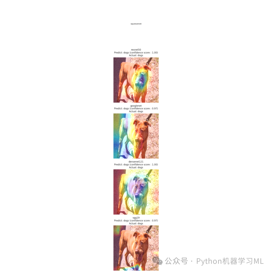
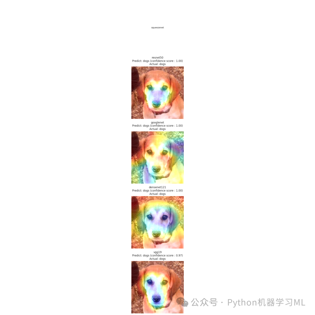
Grad-CAM (Gradient-weighted Class Activation Mapping):

可视化模型关注的图像区域，解释模型判断依据。
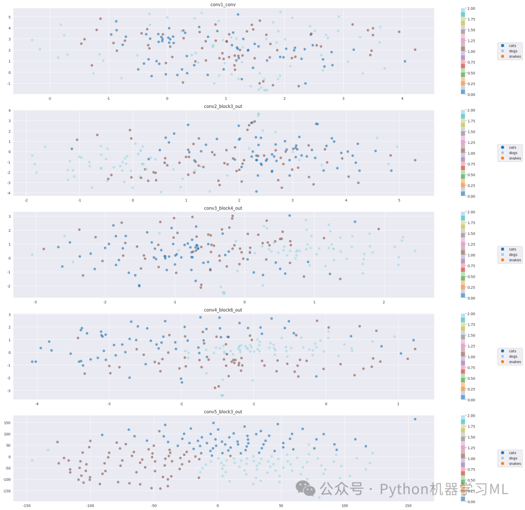
t-SNE (t-distributed Stochastic Neighbor Embedding):

对ResNet50的不同卷积层特征进行降维可视化，观察特征的抽象程度变化，了解模型如何逐步提取图像特征。

第一阶段：导入必要的库和模块

复制代码

# 导入系统库
import os # 用于操作文件和目录
import itertools # 提供高效的循环迭代工具
from PIL import Image # pillow库，用于图像处理

导入数据处理工具`

import numpy as np # 用于数值计算的基础库
import pandas as pd # 用于数据分析和处理的库
import seaborn as sns # 基于matplotlib的数据可视化库
sns.set_style('darkgrid') # 设置seaborn的绘图风格为darkgrid
import matplotlib.pyplot as plt # 绘图库
from sklearn.model_selection import train_test_split # 用于划分训练集和测试集
from tensorflow.keras.layers import BatchNormalization, Activation, Dropout # Keras层组件
from sklearn.metrics import confusion_matrix, classification_report # 用于模型评估的工具

导入深度学习库`

import tensorflow as tf # TensorFlow深度学习框架
from tensorflow import keras # Keras高级API
from tensorflow.keras.models import Sequential # 序贯模型API
from tensorflow.keras.optimizers import Adam, Adamax # 优化器
from tensorflow.keras.preprocessing.image import ImageDataGenerator # 图像数据增强工具
from tensorflow.keras.layers import Conv2D, MaxPooling2D, Flatten, Dense # 卷积神经网络的基本层

print('modules loaded') # 打印提示，表示所有模块已加载完成

可更换为自己的数据集，数据集结构如图。这一阶段的目的是导入项目所需的所有Python库和模块。这些库涵盖了系统操作、数据处理、可视化、机器学习和深度学习等多个方面，为后续的图像分类任务提供必要的工具支持。

第二阶段：数据准备和加载

# 生成训练数据路径和标签
train_data_dir = '2025-3-18公众python机器学习ml-Animals/Animals'# 训练数据目录
filepaths = [] # 存储文件路径的列表
labels = [] # 存储标签的列表

folds = os.listdir(train_data_dir) # 获取训练数据目录下的所有文件夹（每个文件夹代表一个类别）
`

print(folds) # 打印所有类别文件夹（已注释）`

遍历每个类别文件夹，收集文件路径和对应标签`

for fold in folds:
foldpath = os.path.join(train_data_dir, fold) # 构建完整的文件夹路径
filelist = os.listdir(foldpath) # 获取该文件夹下的所有文件
for file in filelist:
fpath = os.path.join(foldpath, file) # 构建完整的文件路径
filepaths.append(fpath) # 添加文件路径到列表
labels.append(fold) # 添加对应的标签到列表

将文件路径和标签合并为一个DataFrame`

Fseries = pd.Series(filepaths, name='filepaths') # 创建文件路径Series
Lseries = pd.Series(labels, name='labels') # 创建标签Series
train_df = pd.concat([Fseries, Lseries], axis=1) # 横向合并为DataFrame

加载测试数据`

test_data_dir = '2025-3-18公众python机器学习ml-Animals/Animals'# 测试数据目录
filepaths = [] # 重置文件路径列表
labels = [] # 重置标签列表

folds = os.listdir(test_data_dir) # 获取测试数据目录下的所有文件夹

遍历每个类别文件夹，收集文件路径和对应标签`

for fold in folds:
`

构建完整的文件夹路径`

fold_path = os.path.join(test_data_dir, fold)
`

确保是目录`

if os.path.isdir(fold_path):
`

获取该文件夹下的所有文件`

file_list = os.listdir(fold_path)
for file in file_list:
`

构建完整的文件路径`

file_path = os.path.join(fold_path, file)
filepaths.append(file_path) # 添加文件路径到列表
labels.append(fold) # 添加对应的标签到列表

将测试数据的文件路径和标签合并为一个DataFrame`

Fseries = pd.Series(filepaths, name='filepaths') # 创建文件路径Series
Lseries = pd.Series(labels, name='labels') # 创建标签Series
test_df = pd.concat([Fseries, Lseries], axis=1) # 横向合并为DataFrame

将测试数据划分为验证集和测试集`

valid_df, test_df = train_test_split(test_df, train_size=0.5, shuffle=True, random_state=123) # 50%作为验证集，50%作为测试集

这一阶段的目的是准备和加载数据。代码首先从指定目录读取训练数据和测试数据，将文件路径和对应的类别标签组织成DataFrame格式。然后将测试数据进一步划分为验证集和测试集，以便在模型训练过程中进行验证和最终评估。

第三阶段：数据生成器配置

复制代码

# 设置裁剪后的图像大小和批次大小
batch_size = 32# 每批处理32张图像
img_size = (224, 224) # 图像调整为224x224像素

创建用于训练、验证和测试的ImageDataGenerator`

tr_gen = ImageDataGenerator() # 训练数据生成器，不进行数据增强
ts_gen = ImageDataGenerator() # 测试数据生成器，不进行数据增强

从DataFrame创建训练数据生成器`

train_gen = tr_gen.flow_from_dataframe(
train_df, # 训练数据DataFrame
x_col='filepaths', # 文件路径列名
y_col='labels', # 标签列名
target_size=img_size, # 目标图像大小
class_mode='categorical', # 多分类模式
color_mode='rgb', # RGB彩色图像
shuffle=True, # 打乱数据
batch_size=batch_size # 批次大小
)

从DataFrame创建验证数据生成器`

valid_gen = ts_gen.flow_from_dataframe(
valid_df, # 验证数据DataFrame
x_col='filepaths', # 文件路径列名
y_col='labels', # 标签列名
target_size=img_size, # 目标图像大小
class_mode='categorical', # 多分类模式
color_mode='rgb', # RGB彩色图像
shuffle=True, # 打乱数据
batch_size=batch_size # 批次大小
)

从DataFrame创建测试数据生成器`

test_gen = ts_gen.flow_from_dataframe(
test_df, # 测试数据DataFrame
x_col='filepaths', # 文件路径列名
y_col='labels', # 标签列名
target_size=img_size, # 目标图像大小
class_mode='categorical', # 多分类模式
color_mode='rgb', # RGB彩色图像
shuffle=False, # 不打乱数据，保持原顺序
batch_size=batch_size # 批次大小
)

获取类别信息`

g_dict = train_gen.class_indices # 获取类别索引字典，形式为{'类别名': 索引}
classes = list(g_dict.keys()) # 获取所有类别名称列表

复制代码

modules loadedFound 3000 validated image filenames belonging to 3 classes.Found 1500 validated image filenames belonging to 3 classes.Found 1500 validated image filenames belonging to 3 classes.

这一阶段的目的是配置数据生成器。代码使用Keras的ImageDataGenerator创建了训练、验证和测试数据的生成器，这些生成器可以从磁盘中按需加载图像，并进行必要的预处理（如调整大小、格式转换等）。这种方式可以有效处理大量图像数据，避免一次性将所有图像加载到内存中。

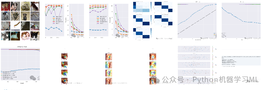
第四阶段：数据可视化

复制代码

# 显示一些带标签的图像样本
images, labels = next(train_gen) # 获取一批训练图像和标签

plt.figure(figsize=(20, 20)) # 创建一个大的图形

显示16张图像`

for i inrange(16):
plt.subplot(4, 4, i + 1) # 创建4x4的子图布局
image = images[i] / 255# 将像素值缩放到0-1范围
plt.imshow(image) # 显示图像
index = np.argmax(labels[i]) # 获取标签的索引（最大值的位置）
class_name = classes[index] # 获取对应的类别名称
plt.title(class_name, color='blue', fontsize=12) # 设置标题为类别名称
plt.axis('off') # 关闭坐标轴
plt.tight_layout() # 调整子图布局
plt.show() # 显示图形

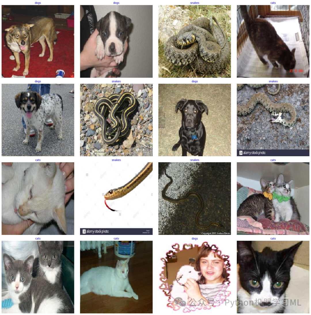
这一阶段的目的是可视化部分训练数据，以便直观了解数据集的内容。代码从训练数据生成器中获取一批图像和标签，然后以4x4的网格布局显示16张图像，每张图像上方标注其类别名称。这有助于确认数据加载正确，并了解数据集中图像的特点。

第五阶段：模型定义

复制代码

from tensorflow.keras.applications import ResNet50, VGG19, DenseNet121
import tensorflow.keras.applications as apps
from tensorflow.keras.layers import GlobalAveragePooling2D
from tensorflow.keras.models import Model

defcreate_model(model_name, input_shape, num_classes):
"""
创建指定的模型架构，增加正则化以避免过拟合
Args:
model_name: 模型名称
input_shape: 输入形状
num_classes: 类别数量
Returns:
编译好的模型
"""
if model_name == 'squeezenet':
`

改进的SqueezeNet实现`

model = Sequential([
`

初始卷积层`

Conv2D(64, 3, strides=2, padding='same', input_shape=input_shape), # 第一个卷积层，64个3x3卷积核
BatchNormalization(), # 批归一化，加速训练并提高稳定性
Activation('relu'), # ReLU激活函数
Dropout(0.2), # 20%的Dropout，防止过拟合
MaxPooling2D(pool_size=3, strides=2, padding='same'), # 最大池化层

`

Fire模块 1`

Fire模块 2`

Conv2D(16, 1, padding='same', kernel_regularizer=tf.keras.regularizers.l2(0.01)), # 瓶颈层，16个1x1卷积核
Activation('relu'), # ReLU激活函数
Conv2D(64, 1, padding='same', kernel_regularizer=tf.keras.regularizers.l2(0.01)), # 扩展层，64个1x1卷积核
Activation('relu'), # ReLU激活函数
Conv2D(64, 3, padding='same', kernel_regularizer=tf.keras.regularizers.l2(0.01)), # 扩展层，64个3x3卷积核
Activation('relu'), # ReLU激活函数
Dropout(0.2), # 20%的Dropout，防止过拟合

GlobalAveragePooling2D(), # 全局平均池化，减少参数量
Dense(num_classes, activation='softmax', kernel_regularizer=tf.keras.regularizers.l2(0.01)) # 输出层，使用softmax激活
])

elif model_name == 'resnet50':
`

使用预训练的ResNet50模型`

base_model = ResNet50(weights='imagenet', include_top=False, input_shape=input_shape) # 加载预训练的ResNet50
`

冻结部分基础层`

for layer in base_model.layers[:-30]: # 冻结除最后30层外的所有层
layer.trainable = False
x = GlobalAveragePooling2D()(base_model.output) # 全局平均池化
x = Dropout(0.5)(x) # 50%的Dropout，防止过拟合
x = Dense(512, activation='relu', kernel_regularizer=tf.keras.regularizers.l2(0.01))(x) # 全连接层
x = Dropout(0.3)(x) # 30%的Dropout，防止过拟合
x = Dense(num_classes, activation='softmax')(x) # 输出层，使用softmax激活
model = Model(inputs=base_model.input, outputs=x) # 创建模型

elif model_name == 'googlenet':
`

使用预训练的InceptionV3模型（GoogleNet的改进版）`

base_model = apps.InceptionV3(weights='imagenet', include_top=False, input_shape=input_shape) # 加载预训练的InceptionV3
`

冻结部分基础层`

for layer in base_model.layers[:-50]: # 冻结除最后50层外的所有层
layer.trainable = False
x = GlobalAveragePooling2D()(base_model.output) # 全局平均池化
x = Dropout(0.5)(x) # 50%的Dropout，防止过拟合
x = Dense(512, activation='relu', kernel_regularizer=tf.keras.regularizers.l2(0.01))(x) # 全连接层
x = BatchNormalization()(x) # 批归一化
x = Dropout(0.3)(x) # 30%的Dropout，防止过拟合
x = Dense(num_classes, activation='softmax')(x) # 输出层，使用softmax激活
model = Model(inputs=base_model.input, outputs=x) # 创建模型

elif model_name == 'densenet121':
`

使用预训练的DenseNet121模型`

base_model = DenseNet121(weights='imagenet', include_top=False, input_shape=input_shape) # 加载预训练的DenseNet121
`

冻结部分基础层`

for layer in base_model.layers[:-40]: # 冻结除最后40层外的所有层
layer.trainable = False
x = GlobalAveragePooling2D()(base_model.output) # 全局平均池化
x = Dropout(0.5)(x) # 50%的Dropout，防止过拟合
x = Dense(512, activation='relu', kernel_regularizer=tf.keras.regularizers.l2(0.01))(x) # 全连接层
x = BatchNormalization()(x) # 批归一化
x = Dropout(0.3)(x) # 30%的Dropout，防止过拟合
x = Dense(num_classes, activation='softmax')(x) # 输出层，使用softmax激活
model = Model(inputs=base_model.input, outputs=x) # 创建模型

elif model_name == 'vgg19':
`

使用预训练的VGG19模型`

base_model = VGG19(weights='imagenet', include_top=False, input_shape=input_shape) # 加载预训练的VGG19
`

冻结部分基础层`

for layer in base_model.layers[:-8]: # 冻结除最后8层外的所有层
layer.trainable = False
x = GlobalAveragePooling2D()(base_model.output) # 全局平均池化
x = Dropout(0.5)(x) # 50%的Dropout，防止过拟合
x = Dense(1024, activation='relu', kernel_regularizer=tf.keras.regularizers.l2(0.01))(x) # 全连接层
x = BatchNormalization()(x) # 批归一化
x = Dropout(0.4)(x) # 40%的Dropout，防止过拟合
x = Dense(512, activation='relu', kernel_regularizer=tf.keras.regularizers.l2(0.01))(x) # 全连接层
x = BatchNormalization()(x) # 批归一化
x = Dropout(0.3)(x) # 30%的Dropout，防止过拟合
x = Dense(num_classes, activation='softmax')(x) # 输出层，使用softmax激活
model = Model(inputs=base_model.input, outputs=x) # 创建模型

`

使用学习率衰减策略`

initial_learning_rate = 0.001# 初始学习率
decay_steps = 1000# 衰减步数
decay_rate = 0.9# 衰减率
learning_rate_schedule = tf.keras.optimizers.schedules.ExponentialDecay(
initial_learning_rate, decay_steps, decay_rate # 指数衰减学习率
)

`

编译模型`

model.compile(
optimizer=Adam(learning_rate=learning_rate_schedule), # Adam优化器，使用学习率衰减
loss='categorical_crossentropy', # 分类交叉熵损失函数
metrics=['accuracy'] # 使用准确率作为评估指标
)

return model

这一阶段的目的是定义不同的深度学习模型架构。代码创建了一个函数，可以根据指定的名称创建不同类型的卷积神经网络模型，包括SqueezeNet、ResNet50、GoogleNet（InceptionV3）、DenseNet121和VGG19。对于预训练模型，代码采用了迁移学习的方法，冻结部分基础层，只训练顶层和部分高级特征层，并添加了正则化技术（如Dropout、L2正则化和批归一化）以防止过拟合。

第六阶段：模型训练和评估

复制代码

# 设置中文显示
plt.rcParams['font.sans-serif'] = ['SimHei'] # 设置中文字体
plt.rcParams['axes.unicode_minus'] = False# 正确显示负号

忽略警告`

import warnings
warnings.filterwarnings('ignore') # 忽略所有警告信息

创建模型列表`

model_names = ['squeezenet', 'resnet50', 'googlenet', 'densenet121', 'vgg19'] # 要训练的模型名称列表
models_history = {} # 存储每个模型的训练历史

训练每个模型`

for model_name in model_names:
print(f"\n训练 {model_name} 模型...") # 打印当前训练的模型名称
model = create_model(model_name, (224, 224, 3), len(classes)) # 创建模型
history = model.fit(
train_gen, # 训练数据生成器
epochs=20, # 训练20个周期
validation_data=valid_gen, # 验证数据
shuffle=False# 不再次打乱数据（数据生成器已经打乱）
)
models_history[model_name] = history # 存储训练历史

`

评估模型`

test_loss, test_accuracy = model.evaluate(test_gen) # 在测试集上评估模型
print(f"{model_name} 测试集准确率: {test_accuracy:.4f}") # 打印测试准确率

这一阶段的目的是训练和评估不同的模型。代码遍历模型名称列表，为每个模型创建相应的架构，然后使用训练数据进行训练，并在验证数据上监控性能。训练完成后，在测试集上评估模型的性能，并打印测试准确率。训练历史被存储在字典中，以便后续分析。

第七阶段：模型性能评估

复制代码

# 导入性能评估工具
from sklearn.metrics import classification_report, roc_auc_score
from sklearn.preprocessing import label_binarize
from sklearn.metrics import accuracy_score, precision_score, recall_score, f1_score

定义一个函数来获取模型性能指标`

defget_model_performance(model, test_gen):
"""
计算模型的各项性能指标

Args:
model: 训练好的模型
test_gen: 测试数据生成器

Returns:
accuracy, precision, recall, f1, auc: 各项性能指标
"""
`

获取预测结果`

y_pred = model.predict(test_gen) # 模型预测
y_pred_classes = np.argmax(y_pred, axis=1) # 获取预测的类别索引
y_true = test_gen.classes # 获取真实的类别索引

`

将真实标签转换为one-hot编码，用于计算AUC`

y_true_bin = label_binarize(y_true, classes=range(len(test_gen.class_indices))) # 将真实标签二值化

`

计算各项指标`

accuracy = accuracy_score(y_true, y_pred_classes) # 准确率
precision = precision_score(y_true, y_pred_classes, average='macro') # 宏平均精确率
recall = recall_score(y_true, y_pred_classes, average='macro') # 宏平均召回率
f1 = f1_score(y_true, y_pred_classes, average='macro') # 宏平均F1分数

`

计算多分类AUC (one-vs-rest)`

auc = roc_auc_score(y_true_bin, y_pred, average='macro', multi_class='ovr') # 多分类ROC AUC

return accuracy, precision, recall, f1, auc

获取每个模型的性能指标`

model_performance = {} # 存储每个模型的性能指标
for model_name, history in models_history.items():
model = history.model # 获取训练好的模型
accuracy, precision, recall, f1, auc = get_model_performance(model, test_gen) # 计算性能指标

`

存储性能指标`

model_performance[model_name] = {
'accuracy': accuracy,
'precision': precision,
'recall': recall,
'f1': f1,
'auc': auc
}

将性能指标转换为DataFrame并格式化显示`

performance_df = pd.DataFrame.from_dict(model_performance, orient='index') # 创建性能指标DataFrame
performance_df = performance_df.round(4) # 保留4位小数

打印性能指标`

print("\n各模型性能指标对比:")
print("="*80)
print(performance_df) # 打印性能指标表格
print("\n指标说明：")
print("准确率(Accuracy): 正确预测的样本数占总样本数的比例")
print("精确率(Precision): 在所有被预测为正类的样本中，真正为正类的比例")
print("召回率(Recall): 在所有真实为正类的样本中，被正确预测为正类的比例")
print("F1分数(F1-Score): 精确率和召回率的调和平均值")
print("AUC值: ROC曲线下的面积，越接近1表示模型性能越好")
print(performance_df.to_csv("各模型性能指标对比.csv")) # 将性能指标保存为CSV文件

这一阶段的目的是全面评估每个模型的性能。代码定义了一个函数，用于计算模型在测试集上的多种性能指标，包括准确率、精确率、召回率、F1分数和AUC值。然后对每个训练好的模型应用这个函数，将结果存储在字典中，并转换为DataFrame进行格式化显示。最后，打印性能指标表格并提供指标说明，同时将结果保存为CSV文件。

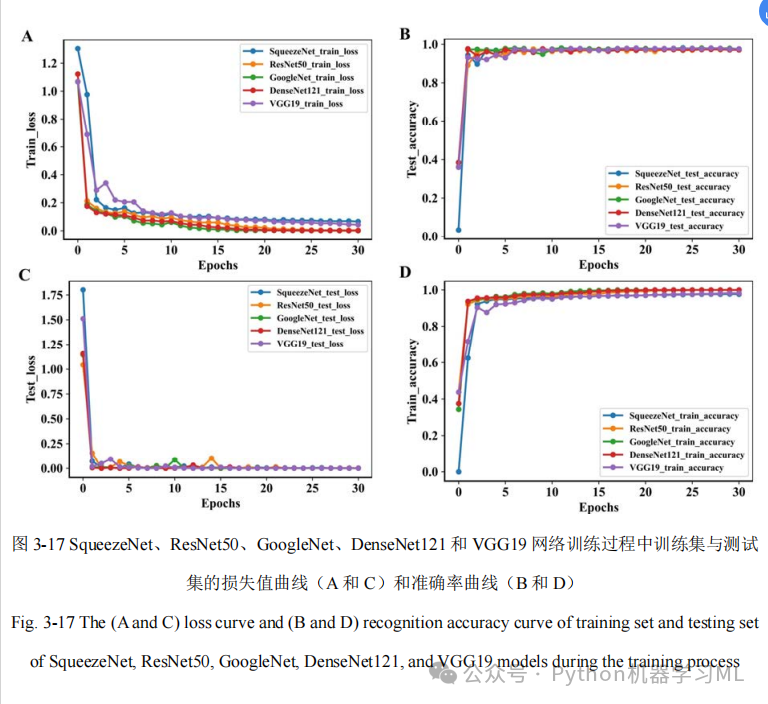
第八阶段：可视化训练过程

复制代码

# 绘制所有模型的对比图
plt.figure(figsize=(15, 5)) # 创建一个宽15高5的图形

训练集准确率对比`

plt.subplot(1, 2, 1) # 创建1行2列的子图，选择第1个
for model_name in models_history:
plt.plot(models_history[model_name].history['accuracy'], label=model_name, marker='o') # 绘制训练准确率曲线
plt.title('Training Accuracy') # 设置标题
plt.xlabel('Epochs') # 设置x轴标签
plt.ylabel('Train_Accuracy') # 设置y轴标签
plt.legend() # 显示图例

训练集损失值对比`

plt.subplot(1, 2, 2) # 创建1行2列的子图，选择第2个
for model_name in models_history:
plt.plot(models_history[model_name].history['loss'], label=model_name, marker='o') # 绘制训练损失曲线
plt.title('Training Loss') # 设置标题
plt.xlabel('Epochs') # 设置x轴标签
plt.ylabel('Train_Loss') # 设置y轴标签
plt.legend() # 显示图例
plt.tight_layout() # 调整子图布局
plt.show() # 显示图形

创建新的图形，用于验证集性能对比`

plt.figure(figsize=(15, 5)) # 创建一个宽15高5的图形

验证集准确率对比`

plt.subplot(1, 2, 1) # 创建1行2列的子图，选择第1个
for model_name in models_history:
plt.plot(models_history[model_name].history['val_accuracy'], label=model_name, marker='o') # 绘制验证准确率曲线
plt.title('Test Accuracy') # 设置标题
plt.xlabel('Epochs') # 设置x轴标签
plt.ylabel('Test_Accuracy') # 设置y轴标签
plt.legend() # 显示图例

验证集损失值对比`

plt.subplot(1, 2, 2) # 创建1行2列的子图，选择第2个
for model_name in models_history:
plt.plot(models_history[model_name].history['val_loss'], label=model_name, marker='o') # 绘制验证损失曲线
plt.title('Test Loss') # 设置标题
plt.xlabel('Epochs') # 设置x轴标签
plt.ylabel('Test_Loss') # 设置y轴标签
plt.legend() # 显示图例

plt.tight_layout() # 调整子图布局
plt.show() # 显示图形

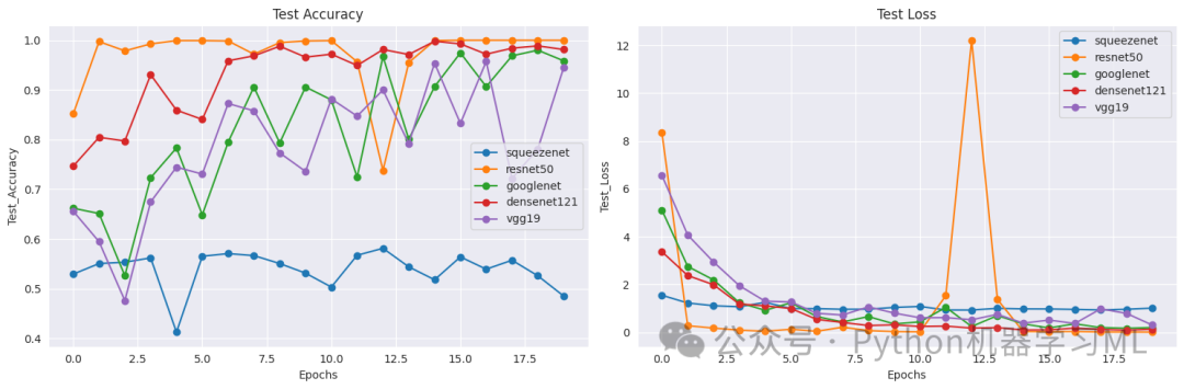
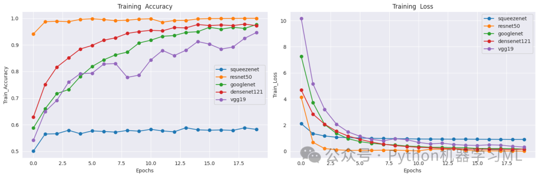
这一阶段的目的是可视化每个模型的训练过程。代码创建了两组图表：第一组显示所有模型在训练集上的准确率和损失曲线，第二组显示所有模型在验证集上的准确率和损失曲线。这些图表可以帮助我们比较不同模型的学习速度、收敛性和泛化能力，从而选择最适合的模型。每个数据点都用圆点标记，使曲线更加清晰可辨。

第九阶段：混淆矩阵分析

复制代码

# 不同模型混淆矩阵热力图对比
from sklearn.metrics import confusion_matrix

定义一个函数来获取混淆矩阵`

defget_confusion_matrix(model, test_gen):
"""
计算模型的混淆矩阵

Args:
model: 训练好的模型
test_gen: 测试数据生成器

Returns:
cm: 混淆矩阵
"""
`

获取预测结果`

y_pred = model.predict(test_gen) # 模型预测
y_pred_classes = np.argmax(y_pred, axis=1) # 获取预测的类别索引
y_true = test_gen.classes # 获取真实的类别索引

`

计算混淆矩阵`

cm = confusion_matrix(y_true, y_pred_classes) # 使用sklearn的confusion_matrix函数

return cm

创建一个字典来存储所有模型`

models = {}
for model_name in model_names:
print(f"\n加载 {model_name} 模型...")

`

创建模型`

model = create_model(model_name, (224, 224, 3), len(classes))

`

加载训练好的权重`

try:
`

从models_history中获取训练好的模型`

trained_model = models_history[model_name].model
`

复制权重到新模型`

model.set_weights(trained_model.get_weights())
print(f"成功加载 {model_name} 模型权重")
except Exception as e:
print(f"加载 {model_name} 模型权重时出错: {str(e)}")
continue

`

将加载好权重的模型添加到字典中`

models[model_name] = model

`

评估模型性能`

print(f"评估 {model_name} 在测试集上的性能...")
test_loss, test_accuracy = model.evaluate(test_gen, verbose=0)
print(f"{model_name} 测试集准确率: {test_accuracy:.4f}")

获取每个模型的混淆矩阵`

confusion_matrices = {}
for model_name, model in models.items():
confusion_matrices[model_name] = get_confusion_matrix(model, test_gen)

绘制混淆矩阵热力图`

plt.figure(figsize=(20, 15)) # 创建一个大的图形
for idx, (model_name, cm) inenumerate(confusion_matrices.items(), 1):
plt.subplot(3, 2, idx) # 创建3行2列的子图布局
sns.heatmap(cm, annot=True, fmt='d', cmap='Blues') # 绘制热力图，显示数值，使用Blues配色
plt.title(f'{model_name}_confusion_matrix') # 设置标题
plt.xlabel('Predicted labels') # 设置x轴标签
plt.ylabel('True labes ') # 设置y轴标签
plt.xticks(range(len(classes)), classes, rotation=45) # 设置x轴刻度为类别名称，旋转45度
plt.yticks(range(len(classes)), classes) # 设置y轴刻度为类别名称

plt.tight_layout() # 调整子图布局
plt.show() # 显示图形

复制代码

加载 squeezenet 模型...成功加载 squeezenet 模型权重评估 squeezenet 在测试集上的性能...squeezenet 测试集准确率: 0.5100加载 resnet50 模型...成功加载 resnet50 模型权重评估 resnet50 在测试集上的性能...resnet50 测试集准确率: 1.0000加载 googlenet 模型...成功加载 googlenet 模型权重评估 googlenet 在测试集上的性能...googlenet 测试集准确率: 0.9667加载 densenet121 模型...成功加载 densenet121 模型权重评估 densenet121 在测试集上的性能...densenet121 测试集准确率: 0.9813加载 vgg19 模型...成功加载 vgg19 模型权重评估 vgg19 在测试集上的性能...vgg19 测试集准确率: 0.9467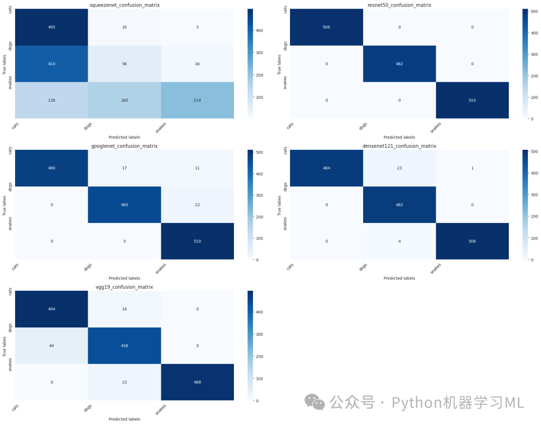

这一阶段的目的是通过混淆矩阵分析每个模型的分类性能。代码首先定义了一个函数，用于计算模型在测试集上的混淆矩阵。然后，它创建了一个新的模型字典，并从之前训练的模型中加载权重。接着，计算每个模型的混淆矩阵，并使用热力图可视化这些矩阵。混淆矩阵可以帮助我们了解每个类别的预测情况，识别模型容易混淆的类别，从而有针对性地改进模型。

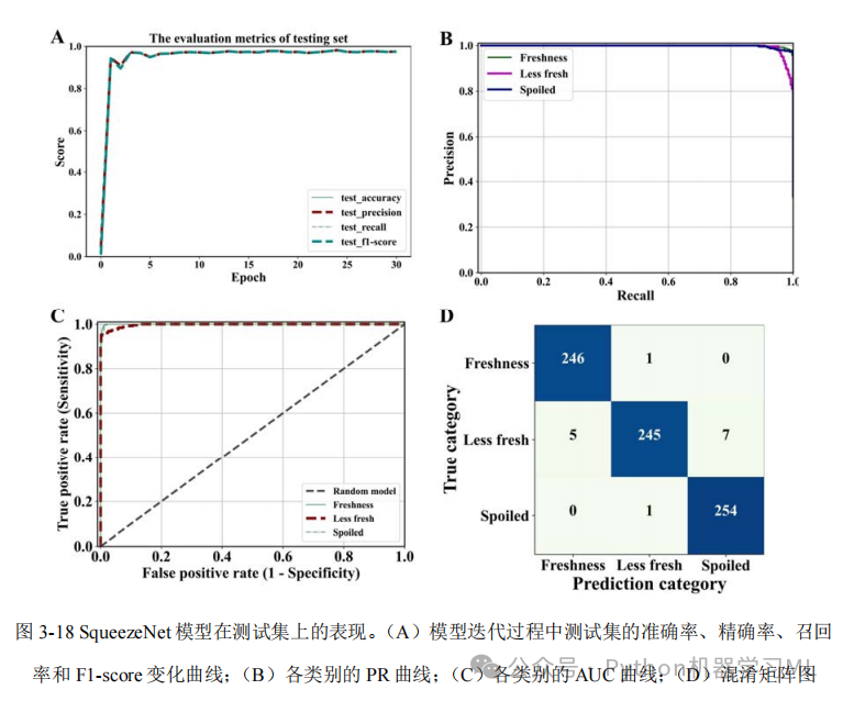
第十阶段：ROC曲线分析

复制代码

# 绘制ROC曲线对比
from sklearn.metrics import roc_curve, auc
from sklearn.preprocessing import label_binarize

defplot_roc_curves(models, test_gen):
"""
绘制所有模型的ROC曲线

Args:
models: 模型字典
test_gen: 测试数据生成器
"""
plt.figure(figsize=(15, 10)) # 创建一个宽15高10的图形

`

获取真实标签`

y_true = test_gen.classes # 获取真实的类别索引
n_classes = len(test_gen.class_indices) # 获取类别数量

`

将真实标签转换为one-hot编码`

y_true_bin = label_binarize(y_true, classes=range(n_classes)) # 将真实标签二值化

`

为每个模型计算并绘制ROC曲线`

for model_name, model in models.items():
`

获取预测概率`

y_pred = model.predict(test_gen) # 模型预测

`

计算每个类别的ROC曲线`

fpr = dict() # 存储假正例率
tpr = dict() # 存储真正例率
roc_auc = dict() # 存储AUC值

`

计算每个类的ROC曲线和AUC值`

for i inrange(n_classes):
fpr[i], tpr[i], _ = roc_curve(y_true_bin[:, i], y_pred[:, i]) # 计算ROC曲线
roc_auc[i] = auc(fpr[i], tpr[i]) # 计算AUC值

`

计算微平均ROC曲线`

fpr["micro"], tpr["micro"], _ = roc_curve(y_true_bin.ravel(), y_pred.ravel()) # 计算微平均ROC曲线
roc_auc["micro"] = auc(fpr["micro"], tpr["micro"]) # 计算微平均AUC值

`

绘制ROC曲线`

plt.plot(
fpr["micro"],
tpr["micro"],
label=f'{model_name} (AUC = {roc_auc["micro"]:.2f})', # 标签包含模型名称和AUC值
lw=2# 线宽
)

`

添加对角线`

plt.plot([0, 1], [0, 1], 'k--', lw=2) # 绘制对角线（随机猜测的基准线）

plt.xlim([0.0, 1.0]) # 设置x轴范围
plt.ylim([0.0, 1.05]) # 设置y轴范围
plt.xlabel('False Positive Rate') # 设置x轴标签
plt.ylabel('True Positive Rate') # 设置y轴标签
plt.title('ROC curves') # 设置标题
plt.legend(loc="lower right") # 显示图例，位置在右下角
plt.grid(True) # 显示网格
plt.show() # 显示图形

使用之前创建的models字典绘制ROC曲线`

plot_roc_curves(models, test_gen)

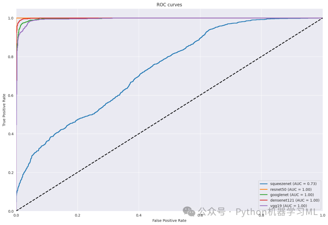
这一阶段的目的是通过ROC曲线分析每个模型的分类性能。代码定义了一个函数，用于计算并绘制每个模型的ROC曲线。ROC曲线展示了模型在不同阈值下的真正例率和假正例率的权衡关系，而曲线下面积（AUC）则是模型性能的一个综合指标。通过比较不同模型的ROC曲线和AUC值，我们可以评估哪个模型在区分不同类别方面表现更好。

第十一阶段：PR曲线分析

复制代码

# 绘制PR曲线对比
from sklearn.metrics import precision_recall_curve, average_precision_score

defplot_pr_curves(models, test_gen):
"""
绘制所有模型的PR曲线

Args:
models: 模型字典
test_gen: 测试数据生成器
"""
plt.figure(figsize=(15, 10)) # 创建一个宽15高10的图形

`

获取真实标签`

y_true = test_gen.classes # 获取真实的类别索引
n_classes = len(test_gen.class_indices) # 获取类别数量

`

将真实标签转换为one-hot编码`

y_true_bin = label_binarize(y_true, classes=range(n_classes)) # 将真实标签二值化

`

为每个模型计算并绘制PR曲线`

for model_name, model in models.items():
`

获取预测概率`

y_pred = model.predict(test_gen) # 模型预测

`

计算每个类别的PR曲线`

precision = dict() # 存储精确率
recall = dict() # 存储召回率
average_precision = dict() # 存储平均精确率

`

计算每个类的PR曲线和平均精确率`

for i inrange(n_classes):
precision[i], recall[i], _ = precision_recall_curve(y_true_bin[:, i], y_pred[:, i]) # 计算PR曲线
average_precision[i] = average_precision_score(y_true_bin[:, i], y_pred[:, i]) # 计算平均精确率

`

计算微平均PR曲线`

precision["micro"], recall["micro"], _ = precision_recall_curve(
y_true_bin.ravel(), y_pred.ravel() # 将多标签问题转换为二分类问题
)
average_precision["micro"] = average_precision_score(
y_true_bin.ravel(), y_pred.ravel(), average="micro"# 计算微平均平均精确率
)

`

绘制PR曲线`

plt.plot(
recall["micro"],
precision["micro"],
label=f'{model_name} (AP = {average_precision["micro"]:.2f})', # 标签包含模型名称和AP值
lw=2# 线宽
)

plt.xlim([0.0, 1.0]) # 设置x轴范围
plt.ylim([0.0, 1.05]) # 设置y轴范围
plt.xlabel('Recall') # 设置x轴标签
plt.ylabel('Precision') # 设置y轴标签
plt.title('PR curves') # 设置标题
plt.legend(loc="lower left") # 显示图例，位置在左下角
plt.grid(True) # 显示网格
plt.show() # 显示图形

打印每个模型的平均精确率`

print("\n各模型的平均精确率(AP):")
print("="*50)
for model_name, model in models.items():
y_pred = model.predict(test_gen) # 模型预测
ap = average_precision_score(y_true_bin.ravel(), y_pred.ravel(), average="micro") # 计算微平均平均精确率
print(f"{model_name}: {ap:.4f}") # 打印模型名称和AP值

绘制每个类别的PR曲线`

defplot_class_pr_curves(models, test_gen, class_names):
"""
为每个类别绘制所有模型的PR曲线

Args:
models: 模型字典
test_gen: 测试数据生成器
class_names: 类别名称列表
"""
n_classes = len(class_names) # 获取类别数量
n_cols = 3# 每行显示3个子图
n_rows = (n_classes + n_cols - 1) // n_cols # 计算需要的行数

plt.figure(figsize=(20, 5*n_rows)) # 创建一个大的图形

`

获取真实标签`

y_true = test_gen.classes # 获取真实的类别索引
y_true_bin = label_binarize(y_true, classes=range(n_classes)) # 将真实标签二值化

for i inrange(n_classes):
plt.subplot(n_rows, n_cols, i+1) # 创建子图

for model_name, model in models.items():
`

获取预测概率`

y_pred = model.predict(test_gen) # 模型预测

`

计算PR曲线`

precision, recall, _ = precision_recall_curve(y_true_bin[:, i], y_pred[:, i]) # 计算PR曲线
ap = average_precision_score(y_true_bin[:, i], y_pred[:, i]) # 计算平均精确率

`

绘制PR曲线`

plt.plot(
recall,
precision,
label=f'{model_name} (AP = {ap:.2f})', # 标签包含模型名称和AP值
lw=2# 线宽
)

plt.xlim([0.0, 1.0]) # 设置x轴范围
plt.ylim([0.0, 1.05]) # 设置y轴范围
plt.xlabel('Recall') # 设置x轴标签
plt.ylabel('Precision') # 设置y轴标签
plt.title(f'catagory: {class_names[i]}') # 设置标题为类别名称
plt.legend(loc="lower left") # 显示图例，位置在左下角
plt.grid(True) # 显示网格

plt.tight_layout() # 调整子图布局
plt.show() # 显示图形

执行PR曲线分析`

print("\n开始绘制PR曲线分析...")
print("="*50)
print("1. 绘制所有模型的整体PR曲线")
plot_pr_curves(models, test_gen)

print("\n2. 绘制每个类别的PR曲线")
plot_class_pr_curves(models, test_gen, classes)

print("\nPR曲线分析说明：")
print("1. PR曲线展示了精确率(Precision)和召回率(Recall)之间的权衡关系")
print("2. 曲线越接近右上角，表示模型性能越好")
print("3. AP(Average Precision)值是PR曲线下的面积，越大越好")
print("4. 对于类别不平衡的数据集，PR曲线比ROC曲线更能反映模型的实际性能")

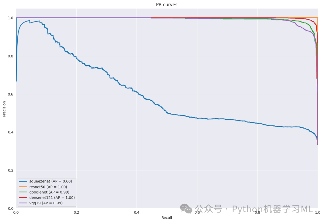
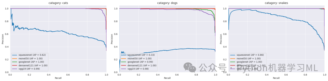
这一阶段的目的是通过PR曲线（精确率-召回率曲线）分析每个模型的分类性能。代码定义了两个函数：一个用于绘制所有模型的整体PR曲线，另一个用于绘制每个类别的PR曲线。PR曲线展示了模型在不同阈值下的精确率和召回率的权衡关系，对于类别不平衡的数据集尤为重要。通过比较不同模型的PR曲线和平均精确率（AP），我们可以评估哪个模型在处理每个类别时表现更好。

第十二阶段：Grad-CAM可视化分析

复制代码

# Grad-CAM可视化分析import tensorflow as tfimport numpy as npimport cv2
def get_img_array(img_array, size):    """    处理输入的图像数组    """    # 如果输入已经是numpy数组，只需要确保尺寸正确    if isinstance(img_array, np.ndarray):        # 调整图像大小        if img_array.shape[:2] != size:            img_array = tf.image.resize(img_array, size)        # 确保批次维度        if len(img_array.shape) == 3:            img_array = np.expand_dims(img_array, axis=0)        return img_array
    # 原始的文件路径处理逻辑    img = tf.keras.preprocessing.image.load_img(img_array, target_size=size)    array = tf.keras.preprocessing.image.img_to_array(img)    array = np.expand_dims(array, axis=0)    return array
def make_gradcam_heatmap(img_array, model, last_conv_layer_name, pred_index=None):    """    生成Grad-CAM热力图    """    # 首先，创建一个模型，将最后一个卷积层和模型的输出作为输出    grad_model = tf.keras.models.Model(        inputs=model.inputs,  # 修改这里：使用model.inputs而不是[model.inputs]        outputs=[            model.get_layer(last_conv_layer_name).output,            model.output        ]    )
    # 计算类别相对于特征图的梯度    with tf.GradientTape() as tape:        conv_outputs, predictions = grad_model(img_array)        if pred_index is None:            pred_index = tf.argmax(predictions[0])        class_channel = predictions[:, pred_index]
    # 获取梯度    grads = tape.gradient(class_channel, conv_outputs)    pooled_grads = tf.reduce_mean(grads, axis=(0, 1, 2))
    # 将特征图与权重相乘    conv_outputs = conv_outputs[0]    heatmap = conv_outputs @ pooled_grads[..., tf.newaxis]    heatmap = tf.squeeze(heatmap)
    # 归一化热力图    heatmap = tf.maximum(heatmap, 0) / tf.math.reduce_max(heatmap)    return heatmap.numpy()
def save_and_display_gradcam(img_array, heatmap, alpha=0.4):    """    将热力图叠加到原始图像上    """    # 确保图像数据在0-255范围内    img = img_array.astype(np.float32)    if img.max() <= 1:        img *= 255
    # 调整热力图大小以匹配原始图像    heatmap = np.uint8(255 * heatmap)    heatmap = cv2.resize(heatmap, (img.shape[1], img.shape[0]))    heatmap = cv2.applyColorMap(heatmap, cv2.COLORMAP_JET)
    # 叠加热力图    superimposed_img = heatmap * alpha + img    superimposed_img = np.clip(superimposed_img, 0, 255).astype(np.uint8)
    return superimposed_img
def visualize_model_attention(model, model_name, img_array, last_conv_layer_name):    """    可视化模型对图像的关注区域    """    # 生成类激活热力图    heatmap = make_gradcam_heatmap(img_array, model, last_conv_layer_name)
    # 叠加热力图到原始图像    superimposed_img = save_and_display_gradcam(img_array[0], heatmap)
    return superimposed_img
def get_last_conv_layer_name(model, model_name):    """    动态获取模型最后一个卷积层的名称    """    # 获取所有层的名称    layer_names = [layer.name for layer in model.layers]
    # 根据不同模型类型查找最后的卷积层    if model_name == 'resnet50':        # 查找最后的残差块        conv_blocks = [name for name in layer_names if 'conv5_block' in name.lower()]        return conv_blocks[-1] if conv_blocks else None    elif model_name == 'googlenet':        # 查找最后的混合层        mixed_layers = [name for name in layer_names if 'mixed' in name.lower()]        return mixed_layers[-1] if mixed_layers else None    elif model_name == 'densenet121':        # 查找最后的密集块        dense_blocks = [name for name in layer_names if 'conv5_block' in name.lower()]        return dense_blocks[-1] if dense_blocks else None    elif model_name == 'vgg19':        # 查找最后的卷积层        conv_layers = [name for name in layer_names if 'conv' in name.lower()]        return conv_layers[-1] if conv_layers else None
    # 如果没有找到匹配的层，返回最后一个卷积层    conv_layers = [name for name in layer_names if 'conv' in name.lower()]    return conv_layers[-1] if conv_layers else None
def visualize_model_predictions(models, test_gen, num_images=5):    """    可视化多个模型对同一图像的预测和关注区域    """    # 获取一些测试图像    test_images = []    batch = next(test_gen)    images = batch[0]  # 图像数组    labels = batch[1]  # 标签
    for i in range(min(num_images, len(images))):        test_images.append((images[i], np.argmax(labels[i])))
    for img_array, true_label_idx in test_images:        plt.figure(figsize=(20, 4*len(models)))        true_label = classes[true_label_idx]
        for idx, (model_name, model) in enumerate(models.items()):            try:                # 获取模型预测                processed_img = get_img_array(img_array, size=(224, 224))                preds = model.predict(processed_img, verbose=0)                pred_label = classes[np.argmax(preds[0])]
                # 动态获取最后一个卷积层的名称                last_conv_layer = get_last_conv_layer_name(model, model_name)                if last_conv_layer is None:                    print(f"警告：无法找到{model_name}的最后一个卷积层")                    continue
                # 生成Grad-CAM可视化                heatmap = make_gradcam_heatmap(processed_img, model, last_conv_layer)                superimposed_img = save_and_display_gradcam(processed_img[0], heatmap)
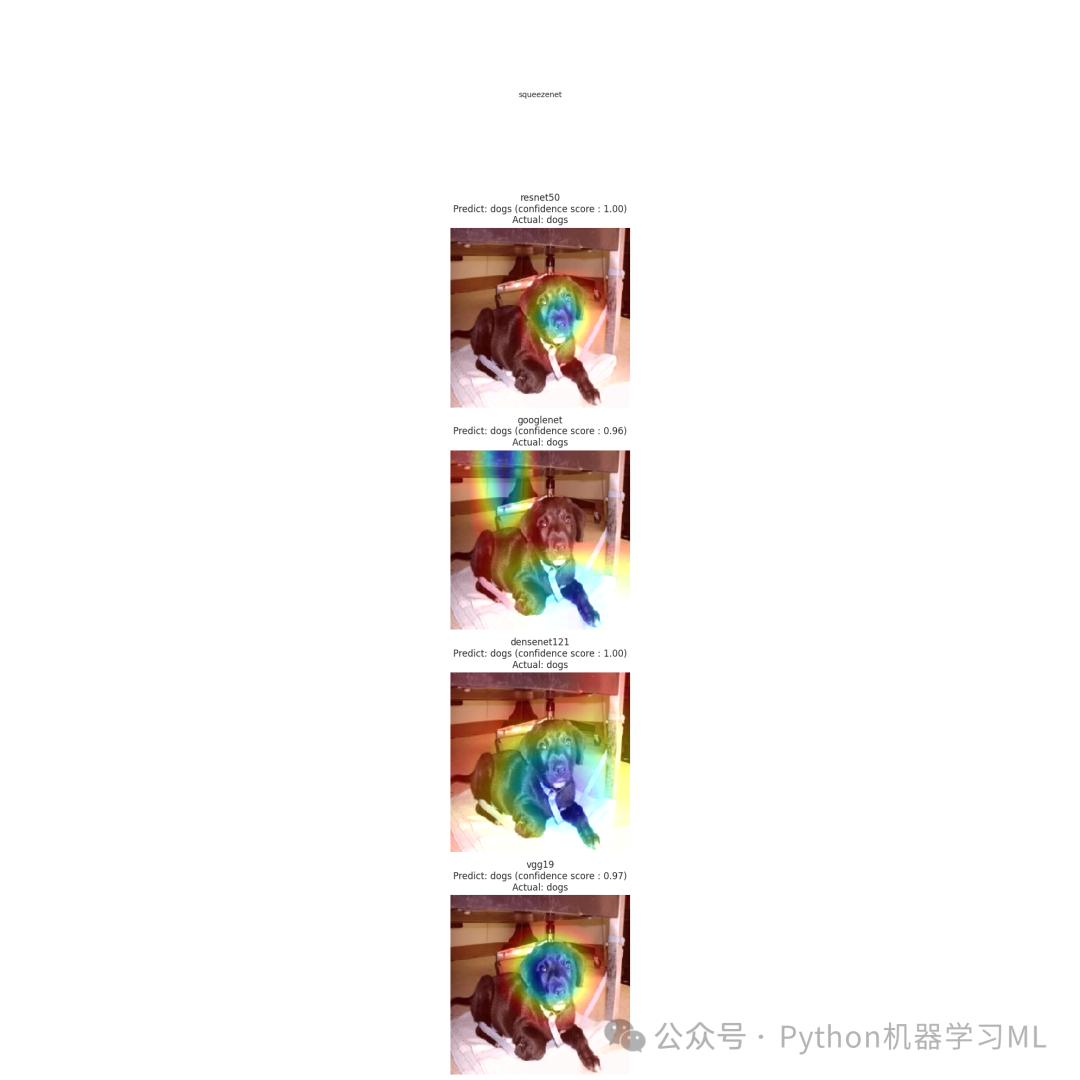
                # 显示结果                plt.subplot(len(models), 1, idx+1)                plt.imshow(superimposed_img)                plt.title(f'{model_name}\nPredict: {pred_label} (confidence score : {np.max(preds[0]):.2f})\nActual: {true_label}')                plt.axis('off')
            except Exception as e:                print(f"警告：处理{model_name}时出错: {str(e)}")                if idx < len(models):                    plt.subplot(len(models), 1, idx+1)                    plt.text(0.5, 0.5, f'{model_name}',                             horizontalalignment='center',                            verticalalignment='center')                    plt.axis('off')                continue
        plt.tight_layout()        plt.show()

# 执行Grad-CAM可视化分析print("\n开始Grad-CAM可视化分析...")print("="*50)print("为每个模型生成类激活热力图，展示模型关注的图像区域")visualize_model_predictions(models, test_gen, num_images=5)
print("\nGrad-CAM分析说明：")print("1. 热力图显示了模型在做出预测时最关注的图像区域")print("2. 红色区域表示模型高度关注的部分，蓝色区域表示较少关注的部分")print("3. 通过比较不同模型的热力图，我们可以理解各个模型的决策依据")print("4. 好的模型通常会关注对象的关键特征，而不是背景或无关区域")

这一阶段的目的是使用Grad-CAM（梯度加权类激活映射）技术可视化每个模型在做出预测时关注的图像区域。代码定义了多个函数，用于生成热力图并将其叠加到原始图像上。对于每个测试图像，代码会显示每个模型的预测结果和关注区域，帮助我们理解模型的决策依据。通过比较不同模型的热力图，我们可以看到哪些模型能够更好地关注对象的关键特征，而不是背景或无关区域。

第十三阶段：t-SNE特征可视化分析

复制代码

#基于Resnet-50各卷积层获得的特征的t-sne方法的可视化
# t-SNE可视化分析from sklearn.manifold import TSNEfrom sklearn.preprocessing import StandardScaler
def get_layer_outputs(model, layer_names, input_data):    """    获取指定层的输出特征    """    # 创建用于提取特征的模型    feature_models = []    for layer_name in layer_names:        feature_model = tf.keras.models.Model(            inputs=model.input,            outputs=model.get_layer(layer_name).output        )        feature_models.append(feature_model)
    # 获取特征    features = []    for feature_model in feature_models:        layer_output = feature_model.predict(input_data, verbose=0)        # 将特征展平为2D        if len(layer_output.shape) > 2:            layer_output = layer_output.reshape(layer_output.shape[0], -1)        features.append(layer_output)
    return features
def perform_tsne(features, n_components=2, perplexity=30):    """    执行t-SNE降维    """    # 标准化特征    scaler = StandardScaler()    features_normalized = scaler.fit_transform(features)
    # 执行t-SNE    tsne = TSNE(n_components=n_components, perplexity=perplexity, random_state=42)    features_tsne = tsne.fit_transform(features_normalized)
    return features_tsne
def visualize_tsne_features(model, test_gen, num_samples=200):  # 减少样本数量    """    可视化ResNet-50不同层的特征分布    """    print("\n开始t-SNE特征可视化分析...")    print("="*50)
    # 收集数据样本    images = []    labels = []    class_counts = {i: 0 for i in range(len(classes))}    samples_per_class = num_samples // len(classes)  # 每个类别更少的样本
    while min(class_counts.values()) < samples_per_class:        batch = next(test_gen)        batch_images, batch_labels = batch        for img, label in zip(batch_images, batch_labels):            label_idx = np.argmax(label)            if class_counts[label_idx] < samples_per_class:                images.append(img)                labels.append(label_idx)                class_counts[label_idx] += 1
    images = np.array(images)    labels = np.array(labels)
    # 选择更少的目标层进行分析    target_layers = [        'conv1_conv',  # 第一个卷积层        'conv2_block3_out',  # 第二个卷积块的输出        'conv3_block4_out',  # 第三个卷积块的输出        'conv4_block6_out',  # 第四个卷积块的输出        'conv5_block3_out'   # 最后的卷积层    ]
    # 获取每一层的特征时使用批处理    print("提取特征...")    batch_size = 32  # 设置较小的批处理大小    features_list = []
    for layer_name in target_layers:        feature_model = tf.keras.models.Model(            inputs=model.input,            outputs=model.get_layer(layer_name).output        )
        # 分批处理数据        features = []        for i in range(0, len(images), batch_size):            batch = images[i:i + batch_size]            layer_output = feature_model.predict(batch, verbose=0)            if len(layer_output.shape) > 2:                layer_output = layer_output.reshape(layer_output.shape[0], -1)            features.append(layer_output)
        features = np.concatenate(features, axis=0)        features_list.append(features)
    # 为每一层执行t-SNE并可视化    plt.figure(figsize=(25, 4*len(target_layers)))  # 增加图形宽度以适应右侧图例
    for idx, (features, layer_name) in enumerate(zip(features_list, target_layers)):        print(f"处理层 {layer_name}...")
        # 执行t-SNE        features_tsne = perform_tsne(features)
        # 创建子图并调整位置以留出图例空间        plt.subplot(len(target_layers), 1, idx+1)        scatter = plt.scatter(features_tsne[:, 0], features_tsne[:, 1],                             c=labels, cmap='tab20', alpha=0.6)        plt.title(f'{layer_name} ')        plt.colorbar(scatter)
        # 添加图例并放置在右侧        legend_elements = [plt.Line2D([0], [0], marker='o', color='w',                                     markerfacecolor=plt.cm.tab20(i/20),                                     label=classes[i], markersize=10)                         for i in range(len(classes))]        plt.legend(handles=legend_elements,                   bbox_to_anchor=(1.15, 0.5),  # 调整到右侧中间位置                  loc='center left',  # 图例左对齐                  borderaxespad=0.)
    plt.tight_layout(rect=[0, 0, 0.85, 1])  # 调整布局，为右侧图例留出空间    plt.show()
    print("\nt-SNE分析说明：")    print("1. 每个点代表一个样本，颜色表示类别")    print("2. 距离相近的点表示特征相似")    print("3. 聚类效果好表示该层能够很好地区分不同类别")    print("4. 从浅层到深层，可以观察特征的抽象程度变化")
# 执行t-SNE分析if 'resnet50' in models:    print("\n开始ResNet-50特征分析...")    visualize_tsne_features(models['resnet50'], test_gen)else:    print("错误：未找到ResNet-50模型")

这段代码的主要作用是使用 t-distributed Stochastic Neighbor Embedding (t-SNE) 技术，对预训练的 ResNet-50 模型在不同卷积层提取的特征进行可视化。通过将高维特征降维到二维空间，并用散点图展示，可以直观地观察到模型不同层对数据的表征能力，以及不同类别样本在特征空间中的分布情况。