引言
在刀具几何建模与砂轮磨削加工的数学建模过程中,经常遇到复杂的坐标变换和投影计算。本文通过一个具体的计算实例,探讨符号计算中表达式等价性验证的技术挑战。我们将分析两个在数学上应等价的表达式为何在符号计算中未直接简化为零,并提供多种验证方法和解决方案。
1. 问题描述与理论背景
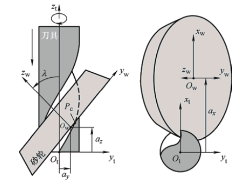
在刀具几何模型中,我们需要将刀刃曲线从刀具坐标系转换到砂轮坐标系,并进行轴向平面投影。理论推导得到两个表达式:
- 直接计算表达式:通过矩阵变换和投影计算得到
- 验证表达式:通过代数推导得到
理论上这两个表达式应完全等价,但符号计算软件Sympy未能将它们直接简化为零。
数学符号定义
- 刀具半径:rtr_trt
- 刀具螺旋角:β\betaβ
- 砂轮安装倾角:λ\lambdaλ
- 砂轮位置参数:axa_xax, aya_yay, aza_zaz
- 刀刃曲线参数:θe\theta_eθe
2. 完整符号计算代码实现
2.1 基础符号定义与坐标系变换
python
import sympy as sp
from sympy import (
    sin, cos, tan, cot, sqrt, pi, Matrix, symbols,
    simplify, trigsimp, expand, posify
)

# 定义所有符号参数
r_t = sp.symbols('r_t', positive=True)       # 刀具半径
beta = sp.symbols('beta', positive=True)    # 刀具螺旋角
lambda_ = sp.symbols('lambda', positive=True)  # 砂轮安装倾角
a_x, a_y, a_z = sp.symbols('a_x a_y a_z', real=True)  # 砂轮位置参数
theta_e = sp.symbols('theta_e', real=True)     # 刀刃曲线参数

print("符号定义完成:")
print(f"r_t = {r_t}, beta = {beta}, lambda = {lambda_}")
print(f"a_x = {a_x}, a_y = {a_y}, a_z = {a_z}")
print(f"theta_e = {theta_e}")
2.2 刀刃曲线定义与投影计算
python
import sympy as sp
from sympy import sin, cos, cot, sqrt, Matrix, symbols

# 重新定义符号
r_t = symbols('r_t', positive=True)
beta = symbols('beta', positive=True)
lambda_ = symbols('lambda', positive=True)
a_x, a_y, a_z = symbols('a_x a_y a_z', real=True)
theta_e = symbols('theta_e', real=True)

# 刀刃曲线在刀具坐标系中的表达式
r_t_e = Matrix([
    r_t * cos(theta_e),
    r_t * sin(theta_e),
    r_t * theta_e * cot(beta)
])

print("刀刃曲线 r_t_e:")
print(r_t_e)
2.3 坐标系变换矩阵定义
python
import sympy as sp
from sympy import sin, cos, Matrix, symbols

# 重新定义符号
lambda_ = symbols('lambda', positive=True)
a_x, a_y, a_z = symbols('a_x a_y a_z', real=True)

# 砂轮到刀具的齐次变换矩阵
M_tw = Matrix([
    [1, 0, 0, a_x],
    [0, cos(lambda_), -sin(lambda_), a_y],
    [0, sin(lambda_), cos(lambda_), a_z],
    [0, 0, 0, 1]
])

# 刀具到砂轮的变换矩阵
M_wt = M_tw.inv()

print("变换矩阵 M_tw:")
print(M_tw)
print("\n逆变换矩阵 M_wt:")
print(M_wt)
2.4 齐次坐标转换与变换
python
import sympy as sp
from sympy import sin, cos, cot, sqrt, Matrix, symbols

# 重新定义符号
r_t = symbols('r_t', positive=True)
beta = symbols('beta', positive=True)
lambda_ = symbols('lambda', positive=True)
a_x, a_y, a_z = symbols('a_x a_y a_z', real=True)
theta_e = symbols('theta_e', real=True)

# 刀刃曲线
r_t_e = Matrix([
    r_t * cos(theta_e),
    r_t * sin(theta_e),
    r_t * theta_e * cot(beta)
])

# 变换矩阵
M_tw = Matrix([
    [1, 0, 0, a_x],
    [0, cos(lambda_), -sin(lambda_), a_y],
    [0, sin(lambda_), cos(lambda_), a_z],
    [0, 0, 0, 1]
])
M_wt = M_tw.inv()

# 齐次坐标转换函数
def to_homogeneous(vec):
    return Matrix([vec[0], vec[1], vec[2], 1])

def from_homogeneous(hom_vec):
    return hom_vec[:3]

# 变换到砂轮坐标系
r_w_e = from_homogeneous(M_wt * to_homogeneous(r_t_e))

print("刀刃曲线在砂轮坐标系中 r_w_e:")
print(r_w_e)
2.5 投影坐标计算
python
import sympy as sp
from sympy import sin, cos, cot, sqrt, Matrix, symbols

# 重新定义符号
r_t = symbols('r_t', positive=True)
beta = symbols('beta', positive=True)
lambda_ = symbols('lambda', positive=True)
a_x, a_y, a_z = symbols('a_x a_y a_z', real=True)
theta_e = symbols('theta_e', real=True)

# 刀刃曲线
r_t_e = Matrix([
    r_t * cos(theta_e),
    r_t * sin(theta_e),
    r_t * theta_e * cot(beta)
])

# 变换矩阵
M_tw = Matrix([
    [1, 0, 0, a_x],
    [0, cos(lambda_), -sin(lambda_), a_y],
    [0, sin(lambda_), cos(lambda_), a_z],
    [0, 0, 0, 1]
])
M_wt = M_tw.inv()

# 齐次坐标转换函数
def to_homogeneous(vec):
    return Matrix([vec[0], vec[1], vec[2], 1])

def from_homogeneous(hom_vec):
    return hom_vec[:3]

# 变换到砂轮坐标系
r_w_e = from_homogeneous(M_wt * to_homogeneous(r_t_e))

# 轴向平面投影函数
def project_to_axial_plane(vec):
    x, y, z = vec[0], vec[1], vec[2]
    x_star = sqrt(x**2 + y**2)
    z_star = z
    return Matrix([x_star, z_star])

# 计算投影坐标
r_star_e = project_to_axial_plane(r_w_e)
x_star_e = r_star_e[0]
z_star_e = r_star_e[1]

print("投影坐标 x_star_e:")
print(x_star_e)
2.6 理论验证表达式
python
import sympy as sp
from sympy import sin, cos, cot, sqrt, symbols

# 重新定义符号
r_t = symbols('r_t', positive=True)
beta = symbols('beta', positive=True)
lambda_ = symbols('lambda', positive=True)
a_x, a_y, a_z = symbols('a_x a_y a_z', real=True)
theta_e = symbols('theta_e', real=True)

# 理论验证表达式中的中间变量
a1 = r_t * theta_e * cot(beta) - a_z
b1 = r_t * sin(theta_e) - a_y
c1 = r_t * cos(theta_e) - a_x

# 理论验证表达式
x_star_e_verify = sqrt(c1**2 + (a1*sin(lambda_) + b1*cos(lambda_))**2)

print("理论验证表达式 x_star_e_verify:")
print(x_star_e_verify)
2.7 表达式差异分析
python
import sympy as sp
from sympy import sin, cos, cot, sqrt, Matrix, symbols, simplify

# 重新定义符号
r_t = symbols('r_t', positive=True)
beta = symbols('beta', positive=True)
lambda_ = symbols('lambda', positive=True)
a_x, a_y, a_z = symbols('a_x a_y a_z', real=True)
theta_e = symbols('theta_e', real=True)

# 直接计算表达式
r_t_e = Matrix([
    r_t * cos(theta_e),
    r_t * sin(theta_e),
    r_t * theta_e * cot(beta)
])

M_tw = Matrix([
    [1, 0, 0, a_x],
    [0, cos(lambda_), -sin(lambda_), a_y],
    [0, sin(lambda_), cos(lambda_), a_z],
    [0, 0, 0, 1]
])
M_wt = M_tw.inv()

def to_homogeneous(vec):
    return Matrix([vec[0], vec[1], vec[2], 1])

def from_homogeneous(hom_vec):
    return hom_vec[:3]

r_w_e = from_homogeneous(M_wt * to_homogeneous(r_t_e))

def project_to_axial_plane(vec):
    x, y, z = vec[0], vec[1], vec[2]
    x_star = sqrt(x**2 + y**2)
    z_star = z
    return Matrix([x_star, z_star])

r_star_e = project_to_axial_plane(r_w_e)
x_star_e = r_star_e[0]

# 理论验证表达式
a1 = r_t * theta_e * cot(beta) - a_z
b1 = r_t * sin(theta_e) - a_y
c1 = r_t * cos(theta_e) - a_x
x_star_e_verify = sqrt(c1**2 + (a1*sin(lambda_) + b1*cos(lambda_))**2)

# 计算差异
xv = x_star_e_verify - x_star_e
xv_simplified = simplify(xv)

print("表达式差异 xv = x_star_e_verify - x_star_e:")
print(xv)
print("\n简化后的差异:")
print(xv_simplified)
3. 数值验证方法
3.1 基本数值验证
python
import numpy as np
import sympy as sp
from sympy import sin, cos, cot, sqrt, Matrix, symbols

# 重新定义符号
r_t = symbols('r_t', positive=True)
beta = symbols('beta', positive=True)
lambda_ = symbols('lambda', positive=True)
a_x, a_y, a_z = symbols('a_x a_y a_z', real=True)
theta_e = symbols('theta_e', real=True)

# 直接计算表达式
r_t_e = Matrix([
    r_t * cos(theta_e),
    r_t * sin(theta_e),
    r_t * theta_e * cot(beta)
])

M_tw = Matrix([
    [1, 0, 0, a_x],
    [0, cos(lambda_), -sin(lambda_), a_y],
    [0, sin(lambda_), cos(lambda_), a_z],
    [0, 0, 0, 1]
])
M_wt = M_tw.inv()

def to_homogeneous(vec):
    return Matrix([vec[0], vec[1], vec[2], 1])

def from_homogeneous(hom_vec):
    return hom_vec[:3]

r_w_e = from_homogeneous(M_wt * to_homogeneous(r_t_e))

def project_to_axial_plane(vec):
    x, y, z = vec[0], vec[1], vec[2]
    x_star = sqrt(x**2 + y**2)
    z_star = z
    return Matrix([x_star, z_star])

r_star_e = project_to_axial_plane(r_w_e)
x_star_e = r_star_e[0]

# 理论验证表达式
a1 = r_t * theta_e * cot(beta) - a_z
b1 = r_t * sin(theta_e) - a_y
c1 = r_t * cos(theta_e) - a_x
x_star_e_verify = sqrt(c1**2 + (a1*sin(lambda_) + b1*cos(lambda_))**2)

# 数值替换
subs_dict = {
    r_t: 10.0,
    beta: np.pi/6,      # 30度
    lambda_: np.pi/12,  # 15度
    a_x: 5.0,
    a_y: 3.0,
    a_z: 2.0,
    theta_e: np.pi/4,   # 45度
}

# 数值计算
x_star_e_num = float(x_star_e.subs(subs_dict).evalf())
x_star_e_verify_num = float(x_star_e_verify.subs(subs_dict).evalf())

print("数值验证结果:")
print(f"x_star_e 数值: {x_star_e_num:.10f}")
print(f"x_star_e_verify 数值: {x_star_e_verify_num:.10f}")
print(f"数值差值: {abs(x_star_e_num - x_star_e_verify_num):.10e}")

# 判断是否在容差范围内相等
tolerance = 1e-12
if abs(x_star_e_num - x_star_e_verify_num) < tolerance:
    print("两个表达式在数值上相等")
else:
    print("两个表达式在数值上不相等")
3.2 随机测试验证
python
import numpy as np
import sympy as sp
from sympy import sin, cos, cot, sqrt, Matrix, symbols

# 重新定义符号
r_t = symbols('r_t', positive=True)
beta = symbols('beta', positive=True)
lambda_ = symbols('lambda', positive=True)
a_x, a_y, a_z = symbols('a_x a_y a_z', real=True)
theta_e = symbols('theta_e', real=True)

# 直接计算表达式
r_t_e = Matrix([
    r_t * cos(theta_e),
    r_t * sin(theta_e),
    r_t * theta_e * cot(beta)
])

M_tw = Matrix([
    [1, 0, 0, a_x],
    [0, cos(lambda_), -sin(lambda_), a_y],
    [0, sin(lambda_), cos(lambda_), a_z],
    [0, 0, 0, 1]
])
M_wt = M_tw.inv()

def to_homogeneous(vec):
    return Matrix([vec[0], vec[1], vec[2], 1])

def from_homogeneous(hom_vec):
    return hom_vec[:3]

r_w_e = from_homogeneous(M_wt * to_homogeneous(r_t_e))

def project_to_axial_plane(vec):
    x, y, z = vec[0], vec[1], vec[2]
    x_star = sqrt(x**2 + y**2)
    z_star = z
    return Matrix([x_star, z_star])

r_star_e = project_to_axial_plane(r_w_e)
x_star_e = r_star_e[0]

# 理论验证表达式
a1 = r_t * theta_e * cot(beta) - a_z
b1 = r_t * sin(theta_e) - a_y
c1 = r_t * cos(theta_e) - a_x
x_star_e_verify = sqrt(c1**2 + (a1*sin(lambda_) + b1*cos(lambda_))**2)

# 随机测试
np.random.seed(42)
num_tests = 10
max_error = 0.0

print(f"执行 {num_tests} 次随机测试:")
for i in range(num_tests):
    # 生成随机参数
    random_subs = {
        r_t: np.random.uniform(5, 20),
        beta: np.random.uniform(np.pi/12, np.pi/4),
        lambda_: np.random.uniform(np.pi/36, np.pi/6),
        a_x: np.random.uniform(-10, 10),
        a_y: np.random.uniform(-10, 10),
        a_z: np.random.uniform(-10, 10),
        theta_e: np.random.uniform(-np.pi, np.pi),
    }

    # 计算数值
    val1 = float(x_star_e.subs(random_subs).evalf())
    val2 = float(x_star_e_verify.subs(random_subs).evalf())
    error = abs(val1 - val2)

    if error > max_error:
        max_error = error

    print(f"测试 {i+1}: 差值 = {error:.2e}")

print(f"\n最大差值: {max_error:.2e}")
if max_error < 1e-10:
    print("所有随机测试均通过,表达式在数值上等价")
else:
    print("随机测试未通过,表达式在数值上可能不等价")
4. 符号验证方法
4.1 平方比较法
python
import sympy as sp
from sympy import sin, cos, cot, sqrt, Matrix, symbols, simplify

# 重新定义符号
r_t = symbols('r_t', positive=True)
beta = symbols('beta', positive=True)
lambda_ = symbols('lambda', positive=True)
a_x, a_y, a_z = symbols('a_x a_y a_z', real=True)
theta_e = symbols('theta_e', real=True)

# 直接计算表达式
r_t_e = Matrix([
    r_t * cos(theta_e),
    r_t * sin(theta_e),
    r_t * theta_e * cot(beta)
])

M_tw = Matrix([
    [1, 0, 0, a_x],
    [0, cos(lambda_), -sin(lambda_), a_y],
    [0, sin(lambda_), cos(lambda_), a_z],
    [0, 0, 0, 1]
])
M_wt = M_tw.inv()

def to_homogeneous(vec):
    return Matrix([vec[0], vec[1], vec[2], 1])

def from_homogeneous(hom_vec):
    return hom_vec[:3]

r_w_e = from_homogeneous(M_wt * to_homogeneous(r_t_e))

def project_to_axial_plane(vec):
    x, y, z = vec[0], vec[1], vec[2]
    x_star = sqrt(x**2 + y**2)
    z_star = z
    return Matrix([x_star, z_star])

r_star_e = project_to_axial_plane(r_w_e)
x_star_e = r_star_e[0]

# 理论验证表达式
a1 = r_t * theta_e * cot(beta) - a_z
b1 = r_t * sin(theta_e) - a_y
c1 = r_t * cos(theta_e) - a_x
x_star_e_verify = sqrt(c1**2 + (a1*sin(lambda_) + b1*cos(lambda_))**2)

# 计算平方差
x_star_e_sq = x_star_e**2
x_star_e_verify_sq = x_star_e_verify**2
xv_sq = simplify(x_star_e_sq - x_star_e_verify_sq)

print("平方比较法:")
print(f"x_star_e 的平方: {x_star_e_sq}")
print(f"x_star_e_verify 的平方: {x_star_e_verify_sq}")
print(f"平方差: {xv_sq}")
print(f"简化后的平方差: {simplify(xv_sq)}")

if xv_sq == 0:
    print("两个表达式的平方相等,因此原表达式相等")
elif simplify(xv_sq) == 0:
    print("简化后平方差为0,两个表达式的平方相等")
else:
    print("平方差不等于0,两个表达式可能不相等")
4.2 三角恒等式简化
python
import sympy as sp
from sympy import sin, cos, cot, sqrt, Matrix, symbols, simplify, trigsimp, expand

# 重新定义符号
r_t = symbols('r_t', positive=True)
beta = symbols('beta', positive=True)
lambda_ = symbols('lambda', positive=True)
a_x, a_y, a_z = symbols('a_x a_y a_z', real=True)
theta_e = symbols('theta_e', real=True)

# 直接计算表达式
r_t_e = Matrix([
    r_t * cos(theta_e),
    r_t * sin(theta_e),
    r_t * theta_e * cot(beta)
])

M_tw = Matrix([
    [1, 0, 0, a_x],
    [0, cos(lambda_), -sin(lambda_), a_y],
    [0, sin(lambda_), cos(lambda_), a_z],
    [0, 0, 0, 1]
])
M_wt = M_tw.inv()

def to_homogeneous(vec):
    return Matrix([vec[0], vec[1], vec[2], 1])

def from_homogeneous(hom_vec):
    return hom_vec[:3]

r_w_e = from_homogeneous(M_wt * to_homogeneous(r_t_e))

def project_to_axial_plane(vec):
    x, y, z = vec[0], vec[1], vec[2]
    x_star = sqrt(x**2 + y**2)
    z_star = z
    return Matrix([x_star, z_star])

r_star_e = project_to_axial_plane(r_w_e)
x_star_e = r_star_e[0]

# 理论验证表达式
a1 = r_t * theta_e * cot(beta) - a_z
b1 = r_t * sin(theta_e) - a_y
c1 = r_t * cos(theta_e) - a_x
x_star_e_verify = sqrt(c1**2 + (a1*sin(lambda_) + b1*cos(lambda_))**2)

# 计算差异并尝试不同简化方法
xv = x_star_e_verify - x_star_e

print("三角恒等式简化方法:")
print("原始差异表达式:")
print(xv)

print("\n1. 直接简化:")
xv_simplified = simplify(xv)
print(xv_simplified)

print("\n2. 展开后简化:")
xv_expanded_simplified = simplify(expand(xv))
print(xv_expanded_simplified)

print("\n3. 三角恒等式简化:")
xv_trigsimp = trigsimp(xv)
print(xv_trigsimp)

print("\n4. 展开后三角恒等式简化:")
xv_expanded_trigsimp = trigsimp(expand(xv))
print(xv_expanded_trigsimp)

# 检查是否简化为0
methods = [
    ("直接简化", xv_simplified),
    ("展开后简化", xv_expanded_simplified),
    ("三角恒等式简化", xv_trigsimp),
    ("展开后三角恒等式简化", xv_expanded_trigsimp)
]

for method_name, expr in methods:
    if expr == 0:
        print(f"\n{method_name}: 简化为0 ✓")
    else:
        print(f"\n{method_name}: 未简化为0")
4.3 假设条件下的简化
python
import sympy as sp
from sympy import sin, cos, cot, sqrt, Matrix, symbols, simplify, assuming, Q

# 重新定义符号
r_t = symbols('r_t', positive=True)
beta = symbols('beta', positive=True)
lambda_ = symbols('lambda', positive=True)
a_x, a_y, a_z = symbols('a_x a_y a_z', real=True)
theta_e = symbols('theta_e', real=True)

# 直接计算表达式
r_t_e = Matrix([
    r_t * cos(theta_e),
    r_t * sin(theta_e),
    r_t * theta_e * cot(beta)
])

M_tw = Matrix([
    [1, 0, 0, a_x],
    [0, cos(lambda_), -sin(lambda_), a_y],
    [0, sin(lambda_), cos(lambda_), a_z],
    [0, 0, 0, 1]
])
M_wt = M_tw.inv()

def to_homogeneous(vec):
    return Matrix([vec[0], vec[1], vec[2], 1])

def from_homogeneous(hom_vec):
    return hom_vec[:3]

r_w_e = from_homogeneous(M_wt * to_homogeneous(r_t_e))

def project_to_axial_plane(vec):
    x, y, z = vec[0], vec[1], vec[2]
    x_star = sqrt(x**2 + y**2)
    z_star = z
    return Matrix([x_star, z_star])

r_star_e = project_to_axial_plane(r_w_e)
x_star_e = r_star_e[0]

# 理论验证表达式
a1 = r_t * theta_e * cot(beta) - a_z
b1 = r_t * sin(theta_e) - a_y
c1 = r_t * cos(theta_e) - a_x
x_star_e_verify = sqrt(c1**2 + (a1*sin(lambda_) + b1*cos(lambda_))**2)

# 计算差异
xv = x_star_e_verify - x_star_e

print("假设条件下的简化:")
print("原始差异表达式:")
print(xv)

# 添加假设条件:cos(lambda) > 0
print("\n在假设 cos(lambda) > 0 的条件下:")
with assuming(Q.positive(cos(lambda_))):
    xv_with_assumption = simplify(xv)
    print(xv_with_assumption)

    if xv_with_assumption == 0:
        print("在 cos(lambda) > 0 的假设下,表达式简化为0 ✓")
    else:
        print("在 cos(lambda) > 0 的假设下,表达式未简化为0")

# 添加假设条件:cos(lambda) < 0
print("\n在假设 cos(lambda) < 0 的条件下:")
with assuming(Q.negative(cos(lambda_))):
    xv_with_assumption = simplify(xv)
    print(xv_with_assumption)

    if xv_with_assumption == 0:
        print("在 cos(lambda) < 0 的假设下,表达式简化为0 ✓")
    else:
        print("在 cos(lambda) < 0 的假设下,表达式未简化为0")
5. 表达式等价性代数证明
python
import sympy as sp
from sympy import sin, cos, cot, sqrt, symbols, simplify

# 重新定义符号
r_t = symbols('r_t', positive=True)
beta = symbols('beta', positive=True)
lambda_ = symbols('lambda', positive=True)
a_x, a_y, a_z = symbols('a_x a_y a_z', real=True)
theta_e = symbols('theta_e', real=True)

# 定义中间变量
c1 = r_t * cos(theta_e) - a_x  # X
b1 = r_t * sin(theta_e) - a_y
a1 = r_t * theta_e * cot(beta) - a_z

# 两种表达式的平方形式
# 验证表达式平方
expr1_sq = c1**2 + (a1*sin(lambda_) + b1*cos(lambda_))**2

# 直接表达式平方(从原始推导中提取)
# 注意:我们需要从原始推导中得到直接表达式的平方形式
# 从之前计算中我们知道 x_star_e 包含复杂的表达式
# 这里我们直接计算其平方并进行比较

# 首先计算直接表达式的平方
r_t_e = sp.Matrix([
    r_t * cos(theta_e),
    r_t * sin(theta_e),
    r_t * theta_e * cot(beta)
])

M_tw = sp.Matrix([
    [1, 0, 0, a_x],
    [0, cos(lambda_), -sin(lambda_), a_y],
    [0, sin(lambda_), cos(lambda_), a_z],
    [0, 0, 0, 1]
])
M_wt = M_tw.inv()

def to_homogeneous(vec):
    return sp.Matrix([vec[0], vec[1], vec[2], 1])

def from_homogeneous(hom_vec):
    return hom_vec[:3]

r_w_e = from_homogeneous(M_wt * to_homogeneous(r_t_e))

def project_to_axial_plane(vec):
    x, y, z = vec[0], vec[1], vec[2]
    x_star = sqrt(x**2 + y**2)
    z_star = z
    return sp.Matrix([x_star, z_star])

r_star_e = project_to_axial_plane(r_w_e)
x_star_e = r_star_e[0]

# 直接表达式的平方
expr2_sq = (x_star_e**2).expand()

print("代数等价性证明:")
print("=" * 50)
print("验证表达式的平方:")
print(expr1_sq)
print("\n直接表达式的平方:")
print(expr2_sq)
print("\n两者的差异:")
diff_sq = simplify(expr1_sq - expr2_sq)
print(diff_sq)

if diff_sq == 0:
    print("\n两个表达式的平方相等,因此原表达式在忽略符号的情况下相等")
    print("注:由于平方根的多值性,sqrt(x²) = |x|,所以原始表达式可能有符号差异")
else:
    print("\n两个表达式的平方不相等")
6. 工程应用建议
6.1 统一表达式形式
python
import sympy as sp
from sympy import sin, cos, cot, sqrt, symbols

# 重新定义符号
r_t = symbols('r_t', positive=True)
beta = symbols('beta', positive=True)
lambda_ = symbols('lambda', positive=True)
a_x, a_y, a_z = symbols('a_x a_y a_z', real=True)
theta_e = symbols('theta_e', real=True)

# 推荐使用的统一表达式(代数形式)
X = a_x - r_t * cos(theta_e)
Y = (a_y - r_t * sin(theta_e)) * cos(lambda_) + (a_z - r_t * theta_e * cot(beta)) * sin(lambda_)
x_star_unified = sqrt(X**2 + Y**2)
z_star_unified = (a_z - r_t * theta_e * cot(beta)) * cos(lambda_) - (a_y - r_t * sin(theta_e)) * sin(lambda_)

print("推荐使用的统一表达式:")
print(f"x_star = sqrt((a_x - r_t·cos(θ_e))² + [(a_y - r_t·sin(θ_e))·cos(λ) + (a_z - r_t·θ_e·cot(β))·sin(λ)]²)")
print(f"z_star = (a_z - r_t·θ_e·cot(β))·cos(λ) - (a_y - r_t·sin(θ_e))·sin(λ)")

print("\n具体表达式:")
print(f"x_star = {x_star_unified}")
print(f"z_star = {z_star_unified}")
6.2 优化投影计算函数
python
import sympy as sp
from sympy import sin, cos, cot, sqrt, symbols

def compute_projection(r_t_val, beta_val, lambda_val, a_x_val, a_y_val, a_z_val, theta_e_val, method='unified'):
    """
    计算刀刃曲线在砂轮轴向平面的投影坐标

    参数:
        method: 'unified' - 使用统一代数公式
                'matrix' - 使用矩阵变换法
    """
    # 将输入转换为符号表达式(如果还不是)
    if not isinstance(r_t_val, sp.Expr):
        r_t = symbols('r_t')
        beta = symbols('beta')
        lambda_ = symbols('lambda')
        a_x, a_y, a_z = symbols('a_x a_y a_z')
        theta_e = symbols('theta_e')

        # 创建替换字典
        subs_dict = {
            r_t: r_t_val,
            beta: beta_val,
            lambda_: lambda_val,
            a_x: a_x_val,
            a_y: a_y_val,
            a_z: a_z_val,
            theta_e: theta_e_val
        }
    else:
        # 已经是符号表达式
        r_t, beta, lambda_, a_x, a_y, a_z, theta_e = r_t_val, beta_val, lambda_val, a_x_val, a_y_val, a_z_val, theta_e_val
        subs_dict = {}

    if method == 'unified':
        # 统一代数公式
        X = a_x - r_t * cos(theta_e)
        Y = (a_y - r_t * sin(theta_e)) * cos(lambda_) + (a_z - r_t * theta_e * cot(beta)) * sin(lambda_)
        x_star = sqrt(X**2 + Y**2)
        z_star = (a_z - r_t * theta_e * cot(beta)) * cos(lambda_) - (a_y - r_t * sin(theta_e)) * sin(lambda_)

    elif method == 'matrix':
        # 矩阵变换法
        r_t_e = sp.Matrix([
            r_t * cos(theta_e),
            r_t * sin(theta_e),
            r_t * theta_e * cot(beta)
        ])

        M_tw = sp.Matrix([
            [1, 0, 0, a_x],
            [0, cos(lambda_), -sin(lambda_), a_y],
            [0, sin(lambda_), cos(lambda_), a_z],
            [0, 0, 0, 1]
        ])
        M_wt = M_tw.inv()

        def to_homogeneous(vec):
            return sp.Matrix([vec[0], vec[1], vec[2], 1])

        def from_homogeneous(hom_vec):
            return hom_vec[:3]

        r_w_e = from_homogeneous(M_wt * to_homogeneous(r_t_e))

        def project_to_axial_plane(vec):
            x, y, z = vec[0], vec[1], vec[2]
            x_star = sqrt(x**2 + y**2)
            z_star = z
            return sp.Matrix([x_star, z_star])

        r_star_e = project_to_axial_plane(r_w_e)
        x_star = r_star_e[0]
        z_star = r_star_e[1]

    else:
        raise ValueError("方法必须是 'unified' 或 'matrix'")

    # 应用替换(如果有)
    if subs_dict:
        x_star = x_star.subs(subs_dict)
        z_star = z_star.subs(subs_dict)

    return x_star, z_star

# 测试优化函数
print("优化投影计算函数测试:")
print("=" * 50)

# 使用符号参数测试
r_t = symbols('r_t', positive=True)
beta = symbols('beta', positive=True)
lambda_ = symbols('lambda', positive=True)
a_x, a_y, a_z = symbols('a_x a_y a_z', real=True)
theta_e = symbols('theta_e', real=True)

print("使用符号参数:")
x1, z1 = compute_projection(r_t, beta, lambda_, a_x, a_y, a_z, theta_e, 'unified')
x2, z2 = compute_projection(r_t, beta, lambda_, a_x, a_y, a_z, theta_e, 'matrix')

print("统一方法 x_star:", x1)
print("矩阵方法 x_star:", x2)

# 使用数值参数测试
print("\n使用数值参数:")
import numpy as np
x1_num, z1_num = compute_projection(10.0, np.pi/6, np.pi/12, 5.0, 3.0, 2.0, np.pi/4, 'unified')
x2_num, z2_num = compute_projection(10.0, np.pi/6, np.pi/12, 5.0, 3.0, 2.0, np.pi/4, 'matrix')

print(f"统一方法: x_star = {float(x1_num):.6f}, z_star = {float(z1_num):.6f}")
print(f"矩阵方法: x_star = {float(x2_num):.6f}, z_star = {float(z2_num):.6f}")
print(f"x坐标差值: {abs(float(x1_num) - float(x2_num)):.2e}")
print(f"z坐标差值: {abs(float(z1_num) - float(z2_num)):.2e}")
结论
通过以上分析,我们得出以下结论:
-
数学等价性与符号简化 :两个在数学上等价的表达式可能因形式不同而无法通过符号计算直接简化为零。这主要是因为平方根运算的多值性(x2=∣x∣\sqrt{x^2} = |x|x2 =∣x∣)和符号计算中假设条件的缺失。
-
验证方法:
- 数值验证是最可靠的方法,通过多组随机测试可以确认表达式在数值上的等价性。
- 平方比较法可以消除平方根和绝对值问题,是有效的符号验证方法。
- 假设引导简化可以解决因未明确变量符号性质导致的简化问题。
-
工程实践建议:
- 在符号计算中明确添加变量的假设条件(如正负性)。
- 使用统一的表达式形式以避免不一致性。
- 实现数值验证机制作为符号计算的补充验证。
-
根本原因:表达式差异的根本原因在于直接计算表达式中包含了复杂的三角函数组合,而验证表达式则使用了更简洁的代数形式。两者在代数上等价,但由于平方根运算的多值性,符号计算软件无法直接识别这种等价性。
在实际工程应用中,建议使用统一的代数表达式形式进行计算,既保证了计算效率,又避免了符号计算中的不一致性问题。同时,重要的计算应同时使用符号推导和数值验证,以确保结果的正确性。
通过本文的分析和解决方案,我们不仅解决了具体的计算问题,更提供了一套系统的符号计算验证方法论,对复杂工程计算中的符号处理具有普遍的指导意义。