最近复现很多DL算法(尤其是涉及到多尺度的情况),经常使用卷积操作,输入参数还需调整,很容易出现维度对不上的情况。方法比较老,有些操作细节不太记得了,这里整理一下。主要整理nn.Conv2d与nn.ConvTranspose2d(转置卷积)操作。
nn.Conv2d的使用
nn.Conv2d 实现二维卷积运算,核心作用是从输入的二维特征图中提取局部特征(比如边缘、纹理、形状等),是卷积神经网络(CNN)的基础组件。可以把卷积理解为:用一个 "过滤器(卷积核)" 在输入图像上滑动,逐位置计算加权求和,最终得到新的特征图。
nn.Conv2d 的初始化参数如下:
python
torch.nn.Conv2d(
    in_channels: int,          # 输入通道数(比如RGB图是3,灰度图是1)
    out_channels: int,         # 输出通道数(卷积核的数量)
    kernel_size: Union[int, Tuple[int, int]],  # 卷积核大小(如3表示3x3,(3,5)表示3行5列)
    stride: Union[int, Tuple[int, int]] = 1,   # 步长(卷积核滑动的步幅,默认1)
    padding: Union[int, Tuple[int, int], str] = 0,  # 填充(边缘补0,默认0;也可设'same'保持尺寸)
    dilation: Union[int, Tuple[int, int]] = 1,  # 空洞卷积的扩张率(默认1,普通卷积)
    groups: int = 1,           # 分组卷积的组数(默认1,普通卷积)
    bias: bool = True,         # 是否添加偏置项(默认True)
    padding_mode: str = 'zeros'# 填充模式(默认补0,还有'reflect'/'replicate'等)
)
基础使用示例:
python
import torch
import torch.nn as nn

# 1. 定义一个Conv2d层:输入3通道(RGB),输出16通道,卷积核3x3,步长1, padding=1(same padding)
conv_layer = nn.Conv2d(in_channels=3, out_channels=16, kernel_size=3, stride=1, padding=1)

# 2. 构造模拟输入:batch_size=2,3通道,高宽为32x32(比如2张32x32的RGB图片)
# 输入形状:[batch_size, in_channels, height, width]
input_tensor = torch.randn(2, 3, 32, 32)

# 3. 执行卷积运算
output_tensor = conv_layer(input_tensor)

# 4. 打印输入输出形状
print(f"输入形状: {input_tensor.shape}")   # 输出:torch.Size([2, 3, 32, 32])
print(f"输出形状: {output_tensor.shape}")  # 输出:torch.Size([2, 16, 32, 32])(padding=1+stride=1,尺寸不变)
这里说明一下输出尺寸计算:
(1)无空洞卷积
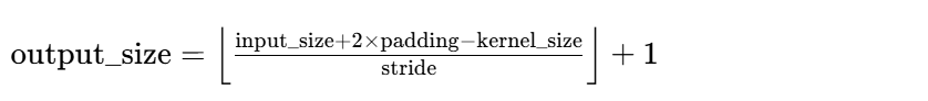
示例验证:
- 输入尺寸 32,kernel_size=3,padding=1,stride=1:
(32+2∗1−3)/1+1=32 → 输出尺寸 32(和输入一致,即 same padding)。 - 若 padding=0,stride=2:向下取整 → 输出尺寸 16。
(2)有空洞卷积
空洞卷积的输出尺寸公式需要加入 dilation 参数,完整公式:
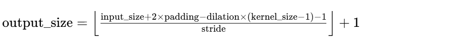
示例验证(空洞卷积)
python
import torch
import torch.nn as nn

# ========== 1. 定义普通卷积(dilation=1)和空洞卷积(dilation=2) ==========
# 普通卷积:3x3核,无空洞
conv_normal = nn.Conv2d(
    in_channels=3, out_channels=16,
    kernel_size=3, stride=1, padding=1, dilation=1
)

# 空洞卷积:3x3核,dilation=2(扩张率2)
# 注意:空洞卷积的padding需要对应调整,否则尺寸会缩小
conv_dilated = nn.Conv2d(
    in_channels=3, out_channels=16,
    kernel_size=3, stride=1, padding=2, dilation=2  # padding=2 保持尺寸不变
)

# ========== 2. 构造输入(单通道、10x10的特征图) ==========
# 输入形状:[batch_size, in_channels, H, W]
input_tensor = torch.randn(2, 3, 32, 32)

# ========== 3. 执行卷积 ==========
out_normal = conv_normal(input_tensor)
out_dilated = conv_dilated(input_tensor)

# ========== 4. 打印结果 ==========
print(f"输入形状: {input_tensor.shape}")       # torch.Size([2, 3, 32, 32])
print(f"普通卷积输出形状: {out_normal.shape}")  # torch.Size([2, 16, 32, 32])
print(f"空洞卷积输出形状: {out_dilated.shape}") # torch.Size([2, 16, 32, 32])

# 查看参数量(两者一致,因为卷积核尺寸都是3x3)
print(f"\n普通卷积参数量: {sum(p.numel() for p in conv_normal.parameters())}")
print(f"空洞卷积参数量: {sum(p.numel() for p in conv_dilated.parameters())}")
nn.ConvTranspose2d的使用
nn.ConvTranspose2d(转置卷积层),它也常被称为 "反卷积"(虽然这个叫法并不严谨),核心作用是对二维特征图进行上采样(放大尺寸),是图像分割、生成对抗网络(GAN)等需要恢复高分辨率特征图任务的核心组件。
nn.ConvTranspose2d 并不是卷积的逆运算(不能完美还原卷积前的输入),而是通过 "补零 + 跨步卷积" 的方式实现特征图的尺寸放大。可以简单理解为:
- 普通卷积(nn.Conv2d):下采样(缩小特征图,提取特征);
- 转置卷积(nn.ConvTranspose2d):上采样(放大特征图,恢复空间维度)。
nn.ConvTranspose2d的核心参数:
python
torch.nn.ConvTranspose2d(
    in_channels: int,          # 输入通道数(和普通卷积一致)
    out_channels: int,         # 输出通道数(和普通卷积一致)
    kernel_size: Union[int, Tuple[int, int]],  # 卷积核大小
    stride: Union[int, Tuple[int, int]] = 1,   # 步长(决定上采样倍数)
    padding: Union[int, Tuple[int, int]] = 0,  # 输入边缘填充(注意:作用和普通卷积相反)
    output_padding: Union[int, Tuple[int, int]] = 0,  # 输出边缘补零(解决尺寸对齐问题)
    groups: int = 1,           # 分组卷积组数
    bias: bool = True,         # 是否加偏置
    dilation: Union[int, Tuple[int, int]] = 1,  # 空洞卷积扩张率
    padding_mode: str = 'zeros'# 填充模式
)
⚠️ 关键区别:output_padding 是转置卷积独有的参数,用于微调输出尺寸,解决步长 > 1 时的尺寸歧义问题。
使用示例:(通过代码对比普通卷积和转置卷积的尺寸变化)
python
import torch
import torch.nn as nn
# ========== 1. 普通卷积(下采样) ==========
# 定义:输入1通道,输出1通道,3x3核,步长2,padding=1
conv = nn.Conv2d(in_channels=1, out_channels=1, kernel_size=3, stride=2, padding=1)
# 构造输入:1个样本,1通道,4x4特征图
x = torch.randn(1, 1, 4, 4)
# 普通卷积输出(下采样)
x_conv = conv(x)
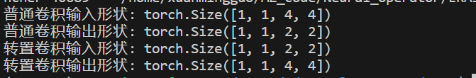
print(f"普通卷积输入形状: {x.shape}") # torch.Size([1, 1, 4, 4])
print(f"普通卷积输出形状: {x_conv.shape}") # torch.Size([1, 1, 2, 2])(步长2导致尺寸减半)
# ========== 2. 转置卷积(上采样) ==========
# 定义:输入1通道,输出1通道,4x4核,步长2,padding=1,output_padding=0
conv_trans = nn.ConvTranspose2d(
in_channels=1, out_channels=1,
kernel_size=4, stride=2, padding=1, output_padding=0
)
# 对普通卷积的输出做转置卷积(上采样)
x_trans = conv_trans(x_conv)
print(f"转置卷积输入形状: {x_conv.shape}") # torch.Size([1, 1, 2, 2])
print(f"转置卷积输出形状: {x_trans.shape}") # torch.Size([1, 1, 4, 4])(还原回4x4)输出结果:
转置卷积的输出尺寸公式是普通卷积的 "逆运算",完整公式:

常见场景的参数搭配(快速上采样)

注意:转置卷积虽然好用,但存在棋盘格效应(Checkerboard Artifact) :由于卷积核的重叠不均,上采样后的特征图会出现类似棋盘格的伪影,这在 GAN 生成图像时尤其明显。
更优的上采样方式:插值 + 普通卷积:先用torch.nn.functional.interpolate 做插值上采样(如双线性插值),再用 1x1 或 3x3 卷积调整通道,避免棋盘格效应。
python
# 更优的上采样方式:插值 + 卷积
x = torch.randn(1, 1, 2, 2)
# 第一步:双线性插值上采样2倍
x_up = nn.functional.interpolate(x, scale_factor=2, mode='bilinear', align_corners=False)
# 第二步:普通卷积调整特征
conv_1x1 = nn.Conv2d(1, 1, kernel_size=1)
x_final = conv_1x1(x_up)
print(x_final.shape)  # torch.Size([1, 1, 4, 4])