给数据“做减法”：PCA与UMAP详解与代码实现

数据降维：PCA主成分分析与UMAP算法的详细解读与实现

ming | 2025.12

在讲解具体的数据降维方法之前，我们必须要明白，什么是数据降维。我们可以从一个熟悉的场景来理解它。

假设你要买一台新手机，面对琳琅满目的品牌和型号，你会如何做出决定？如果是我的话，我可能会去看评测视频或文章，下意识地聚焦于几个核心指标：CPU性能、屏幕素质、电池容量、拍照效果和价格。然后我会综合这些因素来选择一款手机。

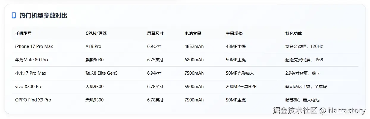
现在，想象你拿到了一张极为详尽的手机参数总表，上面罗列了每一款在售机型的所有数据：

erlang 复制代码

CPU型号，屏幕尺寸（英寸），电池容量（mAh），实测续航时间（小时），充电功率（W），从10%充满电所需时间（分钟），屏幕刷新率（Hz），内存与存储配置（GB），主摄传感器型号，整机重量（g），电源管理系统（PMIC）型号，射频前端（RFFE）模块，音频编解码器型号，搭载的各类传感器，基带芯片版本，图像信号处理器（ISP）型号，参考价格（元）...

上面的这些信息对你挑选手机有帮助吗？当然有，但是太冗余了，有很多信息是没有必要的，其中像"射频前端（RFFE）"这类极其底层的硬件参数，对绝大多数消费者而言，其专业程度和决策相关性都极低，几乎等同于噪声。我相信应该没有人会通过一台手机的射频前端型号来选择手机。这时候，我们就要对这个表进行数据降维了。

数据降维的本质，是对原始数据做一次智能的"信息提纯" 。它并非随意丢弃，而是通过数学变换，将这张庞杂的表格转化为我们能够直观理解 和高效使用的"核心指标看板"；比如上面的"电池容量"和"续航时间"，这两个特征是高度相关的；再比如诸如"射频前端"，"PMIC"这些特征，可能对最终决策影响很小，大多数人都不会关注这个。因此我们可以将这些多余的特征维度去除，只留下最能对我们挑选手机有用的特征即可，这就是数据降维。

在机器学习领域中，一个数据集的特征（维度）动辄成百上千，高维数据不仅会增加计算负担，还容易引发"维度灾难"，导致模型过拟合、泛化能力下降。（因为有很多特征之间高度相关，还有很多特征对当前任务没有什么影响，属于噪声）。

再举一个简单的例子，有如下的一张表：

水果	特征1	特征2	特征3
苹果	0.12	0.25	0.21
菠萝	0.50	0.98	0.62
香蕉	0.01	0.19	0.10
橘子	0.32	0.63	0.43
橙子	0.64	1.24	0.79

表面上，每个水果由三个特征定义，但实际上，所有有效信息都蕴含在"特征1"这一条轴上。特征2和特征3不过是特征1经过简单线性变换后的"影子"。

实际上，特征2 ≈ 特征1 × 2，特征3 ≈ 特征1 + 0.1。这意味着三个特征中存在严格的线性关系，信息是冗余的。

因此在数据降维的时候完全可以把特征2与3删去。

这个例子揭示了数据降维中一个最经典、也最强大的思想：在看似复杂的高维数据中，往往存在着少数几个"隐藏"的主轴，大部分数据变化都沿着这些主轴发生。找到它们，就相当于抓住了数据的本质结构。

当你对数据降维的必要性与核心思想有了基本了解后，下面就开始讲解数据降维领域最经典的算法------主成分分析（PCA），然后用代码实现一遍这个算法。最后再讲解使用一下现代主流数据降维算法UMAP。

注意：下面的内容需要你有一定的线性代数基础和numpy基础才能理解，否则会很难搞清楚PCA究竟做了一件什么事。

一. PCA主成分分析

要深入理解PCA主成分分析，我们首先需要掌握线性代数中的一个核心概念------SVD奇异值分解。如果你对这个概念还不熟悉，不用担心，接下来我会详细解释什么是SVD。

SVD奇异值分解是线性代数中一个极其重要的数学工具，它描述的是，对于任意一个矩阵 <math xmlns="http://www.w3.org/1998/Math/MathML"> A A </math>A(形状为 <math xmlns="http://www.w3.org/1998/Math/MathML"> m × n m \times n </math>m×n)，都能分解成三个矩阵的乘积 <math xmlns="http://www.w3.org/1998/Math/MathML"> A = U S V T A=USV^{T} </math>A=USVT。其中：

<math xmlns="http://www.w3.org/1998/Math/MathML"> U U </math>U是一个 <math xmlns="http://www.w3.org/1998/Math/MathML"> m × m m \times m </math>m×m的正交矩阵（ <math xmlns="http://www.w3.org/1998/Math/MathML"> U T U = I U^T U = I </math>UTU=I）
<math xmlns="http://www.w3.org/1998/Math/MathML"> V T V^{T} </math>VT是一个 <math xmlns="http://www.w3.org/1998/Math/MathML"> n × n n \times n </math>n×n的正交矩阵（ <math xmlns="http://www.w3.org/1998/Math/MathML"> V V T = I V V^T = I </math>VVT=I）
<math xmlns="http://www.w3.org/1998/Math/MathML"> S S </math>S是一个 <math xmlns="http://www.w3.org/1998/Math/MathML"> m × n m \times n </math>m×n的对角矩阵，对角线上的元素称为奇异值，均为正数且通常按降序排列

注意，任意形状的矩阵都可以进行SVD奇异值分解，但是为了方便起见，这里就认为矩阵 <math xmlns="http://www.w3.org/1998/Math/MathML"> A A </math>A是一个方阵(形状为 <math xmlns="http://www.w3.org/1998/Math/MathML"> n × n n \times n </math>n×n)
<math xmlns="http://www.w3.org/1998/Math/MathML" display="block"> A = U S V T = U [ s 1 0 0 0 0 s 2 0 0 ⋮ ⋮ ⋱ ⋮ 0 0 0 s n ] V T ， ( s 1 ≥ s 2 ≥ s 3 ≥ . . . ≥ s n ≥ 0 ) A = USV^{T} = U\begin{bmatrix} s_{1}& 0& 0& 0\\ 0& s_{2}&0 &0 \\ \vdots & \vdots & \ddots &\vdots \\ 0 & 0 & 0 &s_{n} \end{bmatrix} V^T ，\space\space\space (s_{1}\ge s_{2}\ge s_{3}\ge ...\ge s_{n}\ge 0 ) </math>A=USVT=U s10⋮00s2⋮000⋱000⋮sn VT， (s1≥s2≥s3≥...≥sn≥0)

至于为什么任何一个矩阵能分解成三个特定的矩阵 <math xmlns="http://www.w3.org/1998/Math/MathML"> U , S , V T U,S,V^{T} </math>U,S,VT的乘积，这就是数学问题了，SVD奇异值分解有着坚实的数学基础，如果你对证明过程感兴趣，可以自行在互联网上检索。

这里我们亲手实践一下，python的numpy库中有现成的SVD奇异值分解的函数，可以直接调用。

python 复制代码

import numpy as np
# 定义矩阵A
A = np.array([[2.0, 3,  5], 
              [7,  11, 13], 
              [17, 19, 23]])
# 进行SVD奇异值分解
U, s, V_t = np.linalg.svd(A)  
print(U)
print(s)
print(V_t)

python 复制代码

# 输出
# U
array([[-0.15323907, -0.44072023, -0.8844679 ],
       [-0.46548171, -0.75732959,  0.458016  ],
       [-0.87169063,  0.48188958, -0.08909473]])
# s
array([39.37043356,  2.28397225,  0.86742829])
# V_t
array([[-0.466939  , -0.56240524, -0.68239894],
       [ 0.87977217, -0.21755265, -0.42269583],
       [-0.08926865,  0.79772877, -0.5963723 ]])

注意，上面分解的 <math xmlns="http://www.w3.org/1998/Math/MathML"> s s </math>s之所以是一个一维数组而不是我们上面说的对角矩阵，是因为numpy出于存储效率的考虑，只存储有用的部分，因为其它地方都是0，没有必要存储，只存储对角线上的元素，大大提高存储效率。

现在，我们验证一下numpy进行的SVD矩阵分解是否正确，我们试试将 <math xmlns="http://www.w3.org/1998/Math/MathML"> U ， S ， V T U，S，V^{T} </math>U，S，VT进行矩阵乘法，看看结果是不是 <math xmlns="http://www.w3.org/1998/Math/MathML"> A A </math>A。

首先，把 <math xmlns="http://www.w3.org/1998/Math/MathML"> s s </math>s变成对角矩阵 <math xmlns="http://www.w3.org/1998/Math/MathML"> S S </math>S

python 复制代码

# 将s变为二维对角矩阵
S = np.zeros(A.shape)
S[: len(s), : len(s)] = np.diag(s)
print(S)
# 输出
array([[39.37043356,  0.        ,  0.        ],
       [ 0.        ,  2.28397225,  0.        ],
       [ 0.        ,  0.        ,  0.86742829]])

python 复制代码

print(U @ S @ V_t)	# 这里的@符号是矩阵乘法的意思
# 输出
array([[ 2.,  3.,  5.],
       [ 7., 11., 13.],
       [17., 19., 23.]])

完美还原！ 我们可以看到，通过SVD分解后再重新组合，我们得到了原始的矩阵A。这验证了SVD分解的正确性。

虽然我们在示例中使用了numpy的linalg.svd函数，但在处理大规模数据时，我们通常不会直接使用这个函数来实现，因为它很占内存，并且计算量非常大，小型矩阵还好，但是我们实际应用中要处理的矩阵都是成百上千维的。

接下来，我们换一个视角，将矩阵 <math xmlns="http://www.w3.org/1998/Math/MathML"> U U </math>U 的每一列看成一个列向量 <math xmlns="http://www.w3.org/1998/Math/MathML"> p i ⃗ \vec{p_i} </math>pi ，将矩阵 <math xmlns="http://www.w3.org/1998/Math/MathML"> V V </math>V 的每一列看成一个列向量 <math xmlns="http://www.w3.org/1998/Math/MathML"> q i ⃗ \vec{q_i} </math>qi ，那么上面的式子就可以重新表述为：
<math xmlns="http://www.w3.org/1998/Math/MathML" display="block"> A = U S V T = [ p 1 ⃗ , p 2 ⃗ . . . , p n ⃗ ] [ s 1 0 0 0 0 s 2 0 0 ⋮ ⋮ ⋱ ⋮ 0 0 0 s n ] [ q 1 ⃗ T q 2 ⃗ T ⋮ q n ⃗ T ] A = USV^{T} = [\vec{p_{1}},\vec{p_{2}}...,\vec{p_{n}}]\begin{bmatrix} s_{1}& 0& 0& 0\\ 0& s_{2}&0 &0 \\ \vdots & \vdots & \ddots &\vdots \\ 0 & 0 & 0 &s_{n} \end{bmatrix} \begin{bmatrix} \vec{q_{1}}^{T}\\ \vec{q_{2}}^{T}\\ \vdots \\ \vec{q_{n}}^{T} \end{bmatrix} </math>A=USVT=[p1 ,p2 ...,pn ] s10⋮00s2⋮000⋱000⋮sn q1 Tq2 T⋮qn T

现在，我们将这个式子进行展开化简，利用矩阵乘法的分配律，将其拆解为一系列"多项式"之和：
<math xmlns="http://www.w3.org/1998/Math/MathML" display="block"> A = s 1 p 1 ⃗ q 1 ⃗ T + s 2 p 2 ⃗ q 2 ⃗ T + . . . + s n p n ⃗ q n ⃗ T A = s_{1}\vec{p_{1}}\vec{q_{1}}^{T} + s_{2}\vec{p_{2}}\vec{q_{2}}^{T} + ... + s_{n}\vec{p_{n}}\vec{q_{n}}^{T} </math>A=s1p1 q1 T+s2p2 q2 T+...+snpn qn T

请注意，由于列向量 <math xmlns="http://www.w3.org/1998/Math/MathML"> p i ⃗ \vec{p_i} </math>pi 的形状为 <math xmlns="http://www.w3.org/1998/Math/MathML"> ( n , 1 ) (n,1) </math>(n,1)，行向量 <math xmlns="http://www.w3.org/1998/Math/MathML"> q i ⃗ T \vec{q_i}^T </math>qi T 的形状为 <math xmlns="http://www.w3.org/1998/Math/MathML"> ( 1 , n ) (1,n) </math>(1,n)，因此每一项 <math xmlns="http://www.w3.org/1998/Math/MathML"> p i ⃗ q i ⃗ T \vec{p_i}\vec{q_i}^T </math>pi qi T 都是一个 <math xmlns="http://www.w3.org/1998/Math/MathML"> n × n n \times n </math>n×n 的矩阵。而每个奇异值 <math xmlns="http://www.w3.org/1998/Math/MathML"> s i s_i </math>si 则充当了对应子矩阵的权重系数 ，它的大小衡量了该子矩阵在重构原始矩阵 <math xmlns="http://www.w3.org/1998/Math/MathML"> A A </math>A 时的重要性。

由此，我们发现一个重要的洞察：一个复杂的矩阵 <math xmlns="http://www.w3.org/1998/Math/MathML"> A A </math>A，可以被分解为一系列简单（秩为1）矩阵的加权和。

那么，一个自然的想法就产生了：既然每个子矩阵的贡献由权重 <math xmlns="http://www.w3.org/1998/Math/MathML"> s i s_i </math>si 决定，我们是否可以舍弃那些权重非常小的子矩阵，而只用剩下的主要部分来近似原矩阵 <math xmlns="http://www.w3.org/1998/Math/MathML"> A A </math>A 呢？毕竟，权重小的项对最终合成结果的"影响"微乎其微。

答案是肯定的，而这正是SVD用于数据降维的核心思想。 由于奇异值满足 <math xmlns="http://www.w3.org/1998/Math/MathML"> s 1 ≥ s 2 ≥ s 3 ≥ . . . ≥ s n ≥ 0 s_{1} \ge s_{2} \ge s_{3} \ge ... \ge s_{n} \ge 0 </math>s1≥s2≥s3≥...≥sn≥0，通常它们会快速衰减。这意味着前几个奇异值往往包含了矩阵中绝大部分的信息或"能量"。因此，我们可以只保留前几个最大的奇异值及其对应的子矩阵，来得到一个非常优秀的近似。
<math xmlns="http://www.w3.org/1998/Math/MathML" display="block"> A ≈ s 1 p 1 ⃗ q 1 ⃗ T + s 2 p 2 ⃗ q 2 ⃗ T + s 3 p 3 ⃗ q 3 ⃗ T A \approx s_{1}\vec{p_{1}}\vec{q_{1}}^{T} + s_{2}\vec{p_{2}}\vec{q_{2}}^{T} + s_{3}\vec{p_{3}}\vec{q_{3}}^{T} </math>A≈s1p1 q1 T+s2p2 q2 T+s3p3 q3 T

从矩阵运算的角度看，这个近似过程等价于将三个分解矩阵 <math xmlns="http://www.w3.org/1998/Math/MathML"> U , S , V T U, S, V^T </math>U,S,VT 同时进行"截断"：
<math xmlns="http://www.w3.org/1998/Math/MathML" display="block"> A ≈ [ p 1 ⃗ , p 2 ⃗ , p 3 ⃗ ] [ s 1 0 0 0 s 2 0 0 0 s 3 ] [ q 1 ⃗ T q 2 ⃗ T q 3 ⃗ T ] A \approx [\vec{p_{1}},\vec{p_{2}},\vec{p_{3}}]\begin{bmatrix} s_{1}& 0& 0\\ 0& s_{2}&0 \\ 0 & 0 & s_{3} \end{bmatrix} \begin{bmatrix} \vec{q_{1}}^{T}\\ \vec{q_{2}}^{T}\\ \vec{q_{3}}^{T} \end{bmatrix} </math>A≈[p1 ,p2 ,p3 ] s1000s2000s3 q1 Tq2 Tq3 T

如果你不相信，我们可以做一个实验。

我们知道，一张灰度图像本质上就是一个数值矩阵，每个像素值通常在 <math xmlns="http://www.w3.org/1998/Math/MathML"> 0 0 </math>0 到 <math xmlns="http://www.w3.org/1998/Math/MathML"> 255 255 </math>255 之间。

这里，我使用一张大小为 <math xmlns="http://www.w3.org/1998/Math/MathML"> 640 × 640 640 \times 640 </math>640×640 的灰度图像 Frieren.jpg。

现在，我用Python读取这张图像，得到一个形状为 <math xmlns="http://www.w3.org/1998/Math/MathML"> ( 640 , 640 ) (640, 640) </math>(640,640) 的矩阵 <math xmlns="http://www.w3.org/1998/Math/MathML"> A A </math>A，并对其进行奇异值分解（SVD），得到 <math xmlns="http://www.w3.org/1998/Math/MathML"> U , S , V T U, S, V^T </math>U,S,VT。

python 复制代码

import numpy as np
from PIL import Image	# 需要引入pillow库，用来处理图像

# 读取灰度图像
def read_grayscale_image(image_path):
    img = Image.open(image_path).convert('L')
    img_array = np.array(img)
    return img_array

image_path = './Frieren.jpg'
A = read_grayscale_image(image_path)

# 进行完整的SVD分解
U, S, Vt = np.linalg.svd(A)

不推荐使用上面的代码进行SVD分解，效率非常低，下文会有更加高效的SVD分解实现

由于 <math xmlns="http://www.w3.org/1998/Math/MathML"> A A </math>A 是 <math xmlns="http://www.w3.org/1998/Math/MathML"> 640 × 640 640 \times 640 </math>640×640 的矩阵，根据公式 <math xmlns="http://www.w3.org/1998/Math/MathML"> A = ∑ i = 1 640 s i p i ⃗ q i ⃗ T A = \sum_{i=1}^{640} s_{i}\vec{p_{i}}\vec{q_{i}}^{T} </math>A=∑i=1640sipi qi T，它由640个子矩阵相加而成。现在，我们分别进行"截断"近似：

仅使用最大的前8个子矩阵进行重建。
仅使用最大的前30个子矩阵进行重建。
仅使用最大的前80个子矩阵进行重建。

然后，我们观察这些近似结果与原始图像的对比：

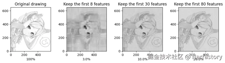
从上图可以清晰地看到：

第一张图是原始图像，由全部640个成分组成。
第二张图仅保留了最核心的8个成分，已经能勾勒出人物的基本轮廓和主要特征，尽管细节模糊且存在块状伪影。
第三张图在轮廓的基础上，恢复了更多的细节和纹理，图像质量显著提升。
第四张图已经能够非常出色地还原原图像，绝大多数细节都得以保留。

这个实验生动地展示了SVD降维的威力：我们仅仅使用了前80个最重要的"特征层"（占总数的12.5%），就实现了对原始数据高达99%以上的视觉保真度。 而剩下的560个子矩阵，其对应的奇异值/权重已经变得非常小，它们所包含的视觉信息大多是极其细微的细节、平滑区域的渐变噪声，或者是人眼不敏感的极高频成分 。舍弃它们可以极大地节省"带宽"或"存储空间"。

如果你已经理解了前面的内容，那么真正的PCA主成分分析对你来说已经触手可及了。

现在假设我们有一个数据集，包含 <math xmlns="http://www.w3.org/1998/Math/MathML"> m m </math>m 个样本，每个样本有 <math xmlns="http://www.w3.org/1998/Math/MathML"> n n </math>n 个特征，可以将其表示为一个形状为 <math xmlns="http://www.w3.org/1998/Math/MathML"> ( m , n ) (m,n) </math>(m,n) 的矩阵 <math xmlns="http://www.w3.org/1998/Math/MathML"> A A </math>A。在进行 PCA 之前，我们通常需要对数据进行标准化处理（这是关键步骤，确保不同量纲的特征具有可比性）。

我们知道对于任意一个矩阵 <math xmlns="http://www.w3.org/1998/Math/MathML"> A A </math>A(形状为 <math xmlns="http://www.w3.org/1998/Math/MathML"> m × n m \times n </math>m×n)，都能分解成三个矩阵的乘积 <math xmlns="http://www.w3.org/1998/Math/MathML"> A = U S V T A=USV^{T} </math>A=USVT。在我们对矩阵 <math xmlns="http://www.w3.org/1998/Math/MathML"> A A </math>A进行分解后，我们得到了如下矩阵：

<math xmlns="http://www.w3.org/1998/Math/MathML"> U U </math>U是一个 <math xmlns="http://www.w3.org/1998/Math/MathML"> m × m m \times m </math>m×m的正交矩阵
<math xmlns="http://www.w3.org/1998/Math/MathML"> V T V^{T} </math>VT是一个 <math xmlns="http://www.w3.org/1998/Math/MathML"> n × n n \times n </math>n×n的正交矩阵
<math xmlns="http://www.w3.org/1998/Math/MathML"> S S </math>S是一个 <math xmlns="http://www.w3.org/1998/Math/MathML"> m × n m \times n </math>m×n的对角矩阵

现在就看你要保留几个奇异值及其对应的子矩阵了，假设你只想保留最大的3个奇异值，那么就要对 <math xmlns="http://www.w3.org/1998/Math/MathML"> U , S , V T U,S,V^{T} </math>U,S,VT进行截断处理；截断后的矩阵如下：

<math xmlns="http://www.w3.org/1998/Math/MathML"> U ^ \hat{U} </math>U^：取 <math xmlns="http://www.w3.org/1998/Math/MathML"> U U </math>U 的前 <math xmlns="http://www.w3.org/1998/Math/MathML"> 3 3 </math>3 列，形状为 <math xmlns="http://www.w3.org/1998/Math/MathML"> m × 3 m \times 3 </math>m×3
<math xmlns="http://www.w3.org/1998/Math/MathML"> S ^ \hat{S} </math>S^：取 <math xmlns="http://www.w3.org/1998/Math/MathML"> S S </math>S 的前 <math xmlns="http://www.w3.org/1998/Math/MathML"> 3 3 </math>3 个奇异值构成的对角矩阵，形状为 <math xmlns="http://www.w3.org/1998/Math/MathML"> 3 × 3 3 \times 3 </math>3×3
<math xmlns="http://www.w3.org/1998/Math/MathML"> V ^ T \hat{V}^T </math>V^T：取 <math xmlns="http://www.w3.org/1998/Math/MathML"> V T V^T </math>VT 的前 <math xmlns="http://www.w3.org/1998/Math/MathML"> 3 3 </math>3 行，形状为 <math xmlns="http://www.w3.org/1998/Math/MathML"> 3 × n 3 \times n </math>3×n

那么降维后的矩阵 <math xmlns="http://www.w3.org/1998/Math/MathML"> A ′ = A ⋅ V ^ A' = A \cdot \hat{V} </math>A′=A⋅V^， <math xmlns="http://www.w3.org/1998/Math/MathML"> A ′ A' </math>A′的形状为 <math xmlns="http://www.w3.org/1998/Math/MathML"> ( m , 3 ) (m,3) </math>(m,3)；其中 <math xmlns="http://www.w3.org/1998/Math/MathML"> V ^ \hat{V} </math>V^ 是 <math xmlns="http://www.w3.org/1998/Math/MathML"> V ^ T \hat{V}^T </math>V^T 的转置

注意，对于等式 <math xmlns="http://www.w3.org/1998/Math/MathML"> A = U S V T A=USV^{T} </math>A=USVT，在等式两边同乘一个 <math xmlns="http://www.w3.org/1998/Math/MathML"> V V </math>V，得到 <math xmlns="http://www.w3.org/1998/Math/MathML"> A V = U S V T V AV=USV^{T}V </math>AV=USVTV；因为 <math xmlns="http://www.w3.org/1998/Math/MathML"> V V </math>V是正交矩阵，所以 <math xmlns="http://www.w3.org/1998/Math/MathML"> V V T = E V V^T = E </math>VVT=E，原式就可以写成 <math xmlns="http://www.w3.org/1998/Math/MathML"> A V = U S AV=US </math>AV=US

所以降维后的矩阵也可以由这个式子得到： <math xmlns="http://www.w3.org/1998/Math/MathML"> A ′ = U ^ ⋅ S ^ A' = \hat{U} \cdot \hat{S} </math>A′=U^⋅S^；两种方式是等价的。

矩阵 <math xmlns="http://www.w3.org/1998/Math/MathML"> A ′ A' </math>A′即为我们通过 PCA 得到降维后的数据表示。这就是PCA主成分分析的数学流程了；到这里就结束了，我们的目标就是得到 <math xmlns="http://www.w3.org/1998/Math/MathML"> A ′ A' </math>A′。我知道你看到这里肯定会很困惑，为什么仅仅通过这样的矩阵乘法就能实现降维？的确，数学是非常有趣的，仅靠白纸黑字和静态的图片可能很难领会到PCA的精髓，PCA需要从几何的角度来理解，这需要你有比较强的线性代数几何基础，如果你看不懂下面的我对PCA的解释，非常推荐看看3Blue1Brown的可视化线性代数教程和可视化PCA教程。

任何两个矩阵相乘，在几何上都可以看作是对空间施加了一次变换------包括拉伸、旋转等操作。具体来说，若矩阵 <math xmlns="http://www.w3.org/1998/Math/MathML"> A A </math>A 与矩阵 <math xmlns="http://www.w3.org/1998/Math/MathML"> B B </math>B 相乘得到 <math xmlns="http://www.w3.org/1998/Math/MathML"> A ⋅ B A \cdot B </math>A⋅B，则相当于将矩阵 <math xmlns="http://www.w3.org/1998/Math/MathML"> A A </math>A 所表示的向量按行（或以行为坐标的向量组）进行 <math xmlns="http://www.w3.org/1998/Math/MathML"> B B </math>B 所定义的线性变换；反过来看，也可以理解为将矩阵 <math xmlns="http://www.w3.org/1998/Math/MathML"> B B </math>B 所表示的向量按列（或以列为坐标的向量组）进行 <math xmlns="http://www.w3.org/1998/Math/MathML"> A A </math>A 所定义的线性变换。

特别地，当变换矩阵为对角矩阵 <math xmlns="http://www.w3.org/1998/Math/MathML"> S S </math>S 时， <math xmlns="http://www.w3.org/1998/Math/MathML"> A ⋅ S A \cdot S </math>A⋅S 意味着对 <math xmlns="http://www.w3.org/1998/Math/MathML"> A A </math>A 的每一行向量，在由 <math xmlns="http://www.w3.org/1998/Math/MathML"> S S </math>S 确定的各个正交轴方向上进行独立的缩放（即纯拉伸，无旋转）。此时， <math xmlns="http://www.w3.org/1998/Math/MathML"> S S </math>S 对角线上的数值就代表对应坐标轴方向上的拉伸因子。而当变换矩阵为正交矩阵 <math xmlns="http://www.w3.org/1998/Math/MathML"> U U </math>U 时， <math xmlns="http://www.w3.org/1998/Math/MathML"> A ⋅ U A \cdot U </math>A⋅U 则表示对 <math xmlns="http://www.w3.org/1998/Math/MathML"> A A </math>A 的行向量进行一种"刚性"旋转变换，不改变向量的长度与彼此间的正交性，因此是保范数且保内积的变换。

基于这样的几何视角，我们可以理解：任何一个矩阵 <math xmlns="http://www.w3.org/1998/Math/MathML"> A A </math>A 都可以通过单位矩阵 <math xmlns="http://www.w3.org/1998/Math/MathML"> E E </math>E 经过一系列变换得到。具体来说，存在正交矩阵 <math xmlns="http://www.w3.org/1998/Math/MathML"> U U </math>U与 <math xmlns="http://www.w3.org/1998/Math/MathML"> V T V^T </math>VT，以及对角矩阵 <math xmlns="http://www.w3.org/1998/Math/MathML"> S S </math>S，使得：
<math xmlns="http://www.w3.org/1998/Math/MathML" display="block"> E ⋅ U ⋅ S ⋅ V T = A E \cdot U \cdot S \cdot V^T = A </math>E⋅U⋅S⋅VT=A

这实际上是奇异值分解的几何表达：从单位矩阵 <math xmlns="http://www.w3.org/1998/Math/MathML"> E E </math>E 出发，先经过 <math xmlns="http://www.w3.org/1998/Math/MathML"> U U </math>U 进行旋转，再经过 <math xmlns="http://www.w3.org/1998/Math/MathML"> S S </math>S 在各正交方向上做不同程度的拉伸，最后通过 <math xmlns="http://www.w3.org/1998/Math/MathML"> V T V^T </math>VT 再做一次旋转，最终得到矩阵 <math xmlns="http://www.w3.org/1998/Math/MathML"> A A </math>A。其中， <math xmlns="http://www.w3.org/1998/Math/MathML"> S S </math>S 的对角元素称为奇异值，它们的大小反映了对应方向上的拉伸强度。奇异值越大，说明该方向上的信息"强度"越高，对数据整体结构的贡献也越大。

值得注意的是，在 <math xmlns="http://www.w3.org/1998/Math/MathML"> E ⋅ U ⋅ S E \cdot U \cdot S </math>E⋅U⋅S 这一步，矩阵的"形态"------即数据在各主要方向上的分布强度------实际上已经确定；最后的 <math xmlns="http://www.w3.org/1998/Math/MathML"> V T V^T </math>VT 变换只是对整个结构做一次整体旋转，并不改变数据的内部相对关系与分布特性。因此，我们完全可以用 <math xmlns="http://www.w3.org/1998/Math/MathML"> U ⋅ S U \cdot S </math>U⋅S 来捕捉 <math xmlns="http://www.w3.org/1998/Math/MathML"> A A </math>A 的核心结构信息。这也意味着，如果我们希望降低数据的维度，可以保留奇异值较大的方向，而舍弃那些奇异值很小的方向，因为它们所包含的信息量很有限，对整体结构的贡献较小。

于是，降维后的近似矩阵可表示为：
<math xmlns="http://www.w3.org/1998/Math/MathML" display="block"> A ′ = U ^ ⋅ S ^ A' = \hat{U} \cdot \hat{S} </math>A′=U^⋅S^

接下来，我们介绍如何在实际应用中高效地对大规模矩阵进行降维操作。这里我们借助 Python 的 sklearn 库来实现。不需要担心你不熟悉这个库，在学习这些强大的工具库（如 SciPy、scikit-learn、Pytorch）时，一个高效的策略是 "按需所学，而非系统通读" 。试图一开始就系统性地掌握一个庞大库的所有内容，很容易陷入大量专业术语的泥潭。更好的方式是，在具体项目中遇到什么需求，再去深入学习该库对应的模块。这能让你始终保持目标清晰，理解也更为深刻。

下面我们就来学习如何使用 sklearn 中提供的 PCA 类，它内部基于高效且稳定的 SVD 实现，只需几行代码即可完成降维。

sklearn库的安装方法为：

bash 复制代码

pip install scikit-learn

使用示例：

python 复制代码

import numpy as np
from sklearn.decomposition import TruncatedSVD

# 示例数据
A = np.array([[3, 4, 3], 
              [5, 1, 6], 
              [7, 2, 9],
              [8, 3, 7]])

# 初始化截断 SVD，保留前 2 个最大的主成分/奇异值
svd = TruncatedSVD(n_components=2)

# 进行数据降维
# 计算出来的result_A就是A'，因为只保留了两个最大的主成分，所以A'矩阵只有两列
result_A = svd.fit_transform(A)  

s = svd.singular_values_	# 奇异值数组
V_t = svd.components_		# 因为只保留了两个最大的主成分，所以V_t矩阵只有两行

# 获取分解结果
print("奇异值s:", s)  
print("V_t:", V_t)  
print("A'",result_A)
# ===输出===
奇异值s: 
[18.43513181  3.20662265]

V_t: 
[[ 0.65528575  0.24759647  0.71365018]
 [ 0.02053089  0.93856832 -0.34448222]]

A': 
[[ 5.09719365  2.78241927]
 [ 7.80592628 -1.02567055]
 [11.50504478 -1.07948712]
 [10.98062664  0.56857653]]

要想通过 <math xmlns="http://www.w3.org/1998/Math/MathML"> A ′ A' </math>A′重建原来的 <math xmlns="http://www.w3.org/1998/Math/MathML"> A A </math>A也很简单，因为 <math xmlns="http://www.w3.org/1998/Math/MathML"> A ′ = A ⋅ V ^ A' = A \cdot \hat{V} </math>A′=A⋅V^，所以 <math xmlns="http://www.w3.org/1998/Math/MathML"> A = A ′ ⋅ V ^ T A = A' \cdot \hat{V}^{T} </math>A=A′⋅V^T；注意，因为 <math xmlns="http://www.w3.org/1998/Math/MathML"> A ′ A' </math>A′是已经降维后的矩阵了，降维过程中丢弃了部分信息，我们无法完全精确地还原原始数据，转换回的新的 <math xmlns="http://www.w3.org/1998/Math/MathML"> A A </math>A后也不再是原来的 <math xmlns="http://www.w3.org/1998/Math/MathML"> A A </math>A了，它肯定与原始 <math xmlns="http://www.w3.org/1998/Math/MathML"> A A </math>A接近，但存在些许差异，这就要看你保留了多少奇异值了。

python 复制代码

new_A = result_A @ V_t
print(new_A)
# ===输出===
[[3.39724391, 3.8735377 , 2.67911918],
 [5.09405433, 0.97005788, 5.92402595],
 [7.51692906, 1.83543602, 8.58244137],
 [7.20712154, 3.25241226, 7.64046165]]

以上就是PCA算法的全部内容。可以看到，PCA的数学原理较为直观，实现也相对容易；但正因如此，它也存在明显的局限性。PCA只能捕捉数据中的线性结构，对于非线性复杂关系的降维效果往往不够理想。此外，PCA对异常值较为敏感，极端值可能会显著影响主成分的方向，从而降低降维结果的质量。

尽管如此，PCA依然是目前最常用和基础的降维方法之一。在实际应用中，很多降维流程会先使用PCA进行初步处理，消除部分噪声与冗余，再结合其他非线性降维方法进一步提取数据结构。

二. UMAP算法

UMAP是一种近年来广受关注的非线性降维算法。与PCA相比，UMAP能够更有效地捕捉数据中复杂的非线性结构，因此在许多实际任务中表现更为强大。

UMAP的理论基础建立在坚实的现代数学框架之上，主要涉及黎曼几何与代数拓扑。它通过构建高维空间中的数据拓扑结构，并尝试在低维空间中保持该结构的本质特征。简单来说，UMAP 的核心思想是在降维过程中尽量保持数据的局部结构------就好像将高维空间中的几何形状"平滑地展开"到低维空间中，形成一张保持相对结构的"解剖图"。

相较于其他非线性降维方法（如 t-SNE），UMAP 的优势非常明显，比如计算效率很高，内存消耗更小，可以处理百万级别的数据等。

尽管UMAP与PCA的最终目标一致------减少数据维度、去除冗余信息，但二者处理数据内在结构的方式有本质不同。下面我们将重点介绍如何使用UMAP工具包进行降维，而不深入其数学细节。

首先需要安装UMAP库

bash 复制代码

pip install umap-learn

为了直观展示UMAP的降维效果，我们以经典的鸢尾花（Iris）数据集为例，演示完整的降维流程。这是一个多分类数据集，包含3个类别（三种鸢尾花品种），每个类别50个样本，共150个样本。每个样本有4个特征：花萼长度、花萼宽度、花瓣长度和花瓣宽度。

鸢尾花（Iris）数据集是sklearn库自带的，只要你之前安装过sklearn库就已经内置了这个数据集了。

python 复制代码

import numpy as np
from sklearn.datasets import load_iris	# 引入鸢尾花数据集

# 加载鸢尾花数据集
iris = load_iris()	
A = iris.data	# 获取特征矩阵，类型为numpy数组
labels = iris.target  # 标签向量，0/1/2分别对应三种鸢尾花
print(A.shape)	# 获取A的形状
print(A[0:10])	# 查看前10个数据

# ===输出===
(150, 4)

[[5.1 3.5 1.4 0.2]
 [4.9 3.  1.4 0.2]
 [4.7 3.2 1.3 0.2]
 [4.6 3.1 1.5 0.2]
 [5.  3.6 1.4 0.2]
 [5.4 3.9 1.7 0.4]
 [4.6 3.4 1.4 0.3]
 [5.  3.4 1.5 0.2]
 [4.4 2.9 1.4 0.2]
 [4.9 3.1 1.5 0.1]]

在获取到样本矩阵后，要对其进行标准化处理（这一步非常关键！PCA中在降维前也是要先进行标准化处理！），之后才能进行降维操作。

python 复制代码

# 进行标准化处理
from sklearn.preprocessing import StandardScaler
scaler = StandardScaler()
scaled_A = scaler.fit_transform(A)    # 对A进行标准化

print(scaled_A[0:10])	# 查看前10个数据

# === 输出 ===
[[-0.90068117  1.01900435 -1.34022653 -1.3154443 ]
 [-1.14301691 -0.13197948 -1.34022653 -1.3154443 ]
 [-1.38535265  0.32841405 -1.39706395 -1.3154443 ]
 [-1.50652052  0.09821729 -1.2833891  -1.3154443 ]
 [-1.02184904  1.24920112 -1.34022653 -1.3154443 ]
 [-0.53717756  1.93979142 -1.16971425 -1.05217993]
 [-1.50652052  0.78880759 -1.34022653 -1.18381211]
 [-1.02184904  0.78880759 -1.2833891  -1.3154443 ]
 [-1.74885626 -0.36217625 -1.34022653 -1.3154443 ]
 [-1.14301691  0.09821729 -1.2833891  -1.44707648]]

接下来进行umap降维：

python 复制代码

import umap

# 初始化 UMAP 模型，设定目标维度为2，固定随机种子以保证可重复性
reducer = umap.UMAP(n_components=2, random_state=42)  
embedding_A = reducer.fit_transform(scaled_A)	# 进行UMAP数据降维

print(embedding_A.shape)	# 查看降维后的数据形状
print(embedding_A[0:10])	# 查看降维后的前10个样本
# === 输出 ===
(150, 2)

[[13.515001   4.9760547]
 [11.787091   3.2109737]
 [11.698444   3.7325902]
 [11.408422   3.5530434]
 [13.728321   5.26629  ]
 [14.782503   5.270304 ]
 [12.758788   4.6392527]
 [13.191469   4.637623 ]
 [11.2218685  3.2424262]
 [11.846259   3.354508 ]]

umap.UMAP()函数的常用参数如下：

参数	作用	推荐范围	影响
`n_neighbors`	控制局部结构的粒度	5~50（默认15）	↗️ 值越大保留全局结构，↘️ 值越小保留局部细节
`min_dist`	控制点的聚集程度	0.001~0.5（默认0.1）	↗️ 值越大点越分散，↘️ 值越小聚类越紧密
`n_components`	降维后的维度	2或3（用于可视化）	一般选2维绘图，3维可交互
`metric`	距离度量方法	'euclidean'（默认）、'cosine'、'manhattan'	根据数据特性选择，例如文本用余弦距离
`n_jobs`	并行计算使用的CPU核心数	根据自己电脑CPU核心数适当配置	加速计算
`random_state`	随机种子	任意整数	固定后可保证每次运行结果一致。

注意：一般情况下umap要保留参数random_state，这样才能保证每次运行结果一致。使得结果可重现。缺点就是它只能在一个CPU核心上运行。若是reducer = umap.UMAP(n_components=2, n_jobs=-1) # -1 表示使用所有CPU核心，就是并行计算，运算速度会大大提升，缺点就是每次降维后的结果可能不同，这种只适合数据可视化的时候使用。

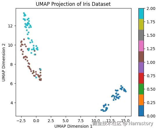
将数据降至二维后，我们可以将这些点绘制在平面直角坐标系中，直观查看降维效果，并用颜色区分不同类别。

python 复制代码

import matplotlib.pyplot as plt	# 引入matplotlib库绘制图表

# 数据可视化（使用散点图）
y = data.target	# 获取每个样本的标签
plt.scatter(embedding[:, 0], embedding[:, 1], c=y, cmap="tab10", s=10)
plt.title("UMAP Projection of Iris Dataset")
plt.xlabel("UMAP Dimension 1")
plt.ylabel("UMAP Dimension 2")
plt.colorbar()
plt.show()

从图中可以看出，降维后的二维数据依然保持了原始数据中三个类别的分离结构，同类样本聚集在一起，不同类之间边界清晰。这说明 UMAP 在降维过程中有效保留了数据的类别信息。

如果你已经用umap降维后的训练集训练了一个模型，那么未来进行推理的时候，新数据如何进行预处理呢？对训练集的数据是如何进行预处理的，那么对新数据就是一样的预处理。

python 复制代码

newData2Predicted = np.array([[4,3,1,0.3]]) # 一个新数据，需要输入到模型中进行运算

# 先将其标准化，再转换为低维，再送到模型中去运算
# 注意不能再创建新的scaler和reducer，必须是之前在处理训练集时定义的scaler和reducer才行。
lowDemensionVersion = reducer.transform(scaler.transform(newData2Predicted))

# 降维后的新数据
print(lowDemensionVersion)

# === 输出 ===
[[11.103776 ,  3.8664804]]

更常用的方法是本地化保存这两个预处理函数scaler和reducer

python 复制代码

import joblib
# 本地化数据预处理模型，将其保存为本地文件
joblib.dump(scaler, 'scaler.pkl')
joblib.dump(reducer, "reducer.pkl")

python 复制代码

newData2Predicted = np.array([[4, 3, 1, 0.3]])  # 一个新数据

# 需要使用的时候再通过加载预处理模型来对其进行预处理
savedScaler = joblib.load('./scaler.pkl')
savedReducer = joblib.load('./reducer.pkl')
newLowDemensionVersion = savedReducer.transform(savedScaler.transform(newData2Predicted))
print(newLowDemensionVersion)

# === 输出 ===
[[11.103776 ,  3.8664804]]