基于深度学习的车牌识别系统

基于深度学习的车牌识别系统

摘要

车牌识别（License Plate Recognition, LPR）作为计算机视觉领域的重要应用，在智能交通、安防监控、智慧城市等领域发挥着关键作用。本文详细介绍了一个基于深度学习的完整车牌识别系统，涵盖车辆检测、车牌定位、字符识别三大核心模块，使用PyTorch、OpenCV和PyQt5等技术栈实现。文章将从技术原理、代码实现、系统优化到实际应用进行全面剖析，为读者提供完整的项目实践指南。

关键词：车牌识别、深度学习、YOLOv3、RetinaNet、LPRNet、PyTorch、OpenCV

---

一、引言

1.1 车牌识别的背景与意义

随着人工智能技术的快速发展，车牌识别技术已经从传统图像处理方法演进到基于深度学习的智能识别阶段。车牌识别系统在以下场景中具有重要应用价值：

• 智能交通管理：交通违章监控、ETC收费系统、停车场管理
• 安防监控：车辆追踪、黑名单识别、出入控制
• 商业应用：智慧园区、小区门禁、物流管理
• 数据分析：车流量统计、出行模式分析、交通规划

1.2 技术发展历程

车牌识别技术的发展经历了三个阶段：

1. 传统图像处理阶段（2000年前）：基于边缘检测、颜色分割、模板匹配等方法
2. 机器学习阶段（2000-2015年）：结合特征提取和分类器（SVM、AdaBoost等）
3. 深度学习阶段（2015年至今）：端到端的深度神经网络方法

1.3 本文贡献

本文的主要贡献包括：

• 提供完整的车牌识别系统实现方案
• 详细解析各模块的技术原理和代码实现
• 分享实际开发中的问题解决方案
• 提供系统优化和部署建议

---

二、系统架构设计

2.1 整体架构

我们的车牌识别系统采用模块化设计，主要包括以下三个核心模块：

输入图像/视频流
    ↓
车辆检测模块（YOLOv3-tiny）
    ↓
车牌定位模块（RetinaNet）
    ↓
字符识别模块（LPRNet）
    ↓
识别结果输出

2.2 技术选型依据

2.2.1 车辆检测模块选择YOLOv3-tiny的原因

YOLOv3-tiny作为YOLO系列的轻量级版本，在精度和速度之间取得了良好平衡：

• 实时性要求：车牌识别系统通常需要实时处理视频流
• 计算资源限制：在边缘设备上部署需要轻量级模型
• 精度保证：相比其他轻量级模型，YOLOv3-tiny在车辆检测任务上表现优异

2.2.2 车牌定位模块选择RetinaNet的原因

RetinaNet在处理小目标检测任务上具有优势：

• 特征金字塔网络（FPN）：有效处理多尺度目标
• Focal Loss：解决正负样本不平衡问题
• 高精度定位：对车牌这种小尺寸目标检测效果好

2.2.3 字符识别模块选择LPRNet的原因

LPRNet是专门为车牌字符识别设计的网络：

• 端到端设计：无需字符分割，直接输出识别结果
• 轻量级架构：适合实时应用场景
• 多语言支持：支持中英文混合车牌识别

2.3 开发环境配置

2.3.1 硬件要求

# 推荐配置
CPU: Intel i7 或同等性能以上
GPU: NVIDIA GTX 1060 6GB 或更高
内存: 16GB 或以上
存储: SSD 256GB 或以上

2.3.2 软件环境

# 核心依赖库
Python == 3.8.0
PyTorch == 1.7.1
TorchVision == 0.8.2
OpenCV == 4.5.1
PyQt5 == 5.15.4
CUDA == 11.0 (可选，GPU加速)

2.3.3 环境安装步骤

# 创建虚拟环境
conda create -n alpr python=3.8
conda activate alpr

# 安装PyTorch (CPU版本)
pip install torch==1.7.1+cpu torchvision==0.8.2+cpu -f https://download.pytorch.org/whl/torch_stable.html

# 安装其他依赖
pip install opencv-python==4.5.1.48
pip install PyQt5==5.15.4
pip install pillow==8.1.0
pip install numpy==1.19.5

# 如果使用GPU，安装CUDA版本
pip install torch==1.7.1+cu110 torchvision==0.8.2+cu110 -f https://download.pytorch.org/whl/torch_stable.html

---

三、车辆检测模块实现

3.1 YOLOv3-tiny原理详解

YOLOv3-tiny是YOLOv3的简化版本，主要特点包括：

3.1.1 网络结构

YOLOv3-tiny使用更少的卷积层和特征图，网络结构如下：

# 简化的网络结构
Input: 416×416×3
    ↓
Darknet-19 Tiny (13个卷积层)
    ↓
两个检测头（13×13和26×26）
    ↓
边界框预测

3.1.2 检测原理

YOLO将检测任务转化为回归问题：

• 网格划分：将输入图像划分为S×S的网格
• 边界框预测：每个网格预测B个边界框和置信度
• 类别预测：每个边界框预测C个类别的概率

3.1.3 损失函数

YOLOv3-tiny的损失函数包含三个部分：

Loss = λ_coord × 坐标损失 + λ_obj × 置信度损失 + λ_noobj × 非目标损失 + 类别损失

3.2 代码实现解析

3.2.1 模型定义

import torch
import torch.nn as nn

class YOLOv3Tiny(nn.Module):
    def __init__(self, num_classes=80):
        super(YOLOv3Tiny, self).__init__()
        self.num_classes = num_classes
        
        # 定义网络层
        self.layers = nn.Sequential(
            # 第一个卷积块
            ConvBlock(3, 16, 3, 1, 1),
            nn.MaxPool2d(2, 2),
            
            # 第二个卷积块
            ConvBlock(16, 32, 3, 1, 1),
            nn.MaxPool2d(2, 2),
            
            # 更多卷积层...
            # 完整的网络结构定义
        )
        
        # 检测头
        self.detection_heads = nn.ModuleList([
            DetectionHead(256, num_classes),  # 13×13检测头
            DetectionHead(128, num_classes)   # 26×26检测头
        ])
    
    def forward(self, x):
        # 前向传播逻辑
        features = []
        for layer in self.layers:
            x = layer(x)
            if isinstance(layer, nn.MaxPool2d):
                features.append(x)
        
        # 检测头输出
        outputs = []
        for i, head in enumerate(self.detection_heads):
            output = head(features[i])
            outputs.append(output)
        
        return outputs

class ConvBlock(nn.Module):
    """卷积块：卷积 + 批归一化 + LeakyReLU"""
    def __init__(self, in_channels, out_channels, kernel_size, stride, padding):
        super(ConvBlock, self).__init__()
        self.conv = nn.Conv2d(in_channels, out_channels, kernel_size, stride, padding, bias=False)
        self.bn = nn.BatchNorm2d(out_channels)
        self.activation = nn.LeakyReLU(0.1)
    
    def forward(self, x):
        return self.activation(self.bn(self.conv(x)))

3.2.2 数据预处理

import cv2
import numpy as np

def preprocess_image(image, target_size=416):
    """图像预处理函数"""
    # 获取原始尺寸
    h, w = image.shape[:2]
    
    # 计算缩放比例
    scale = min(target_size / w, target_size / h)
    nw, nh = int(scale * w), int(scale * h)
    
    # 缩放图像
    resized = cv2.resize(image, (nw, nh))
    
    # 创建填充图像
    padded = np.full((target_size, target_size, 3), 128, dtype=np.uint8)
    
    # 计算填充位置
    dx = (target_size - nw) // 2
    dy = (target_size - nh) // 2
    
    # 填充图像
    padded[dy:dy+nh, dx:dx+nw] = resized
    
    # 归一化
    padded = padded.astype(np.float32) / 255.0
    
    # 调整维度顺序 (H,W,C) -> (C,H,W)
    padded = padded.transpose(2, 0, 1)
    
    return padded, (scale, dx, dy, w, h)

def postprocess_detection(outputs, preprocess_info, confidence_threshold=0.5, nms_threshold=0.4):
    """后处理检测结果"""
    scale, dx, dy, orig_w, orig_h = preprocess_info
    
    detections = []
    
    for output in outputs:
        # 过滤低置信度检测
        mask = output[..., 4] > confidence_threshold
        filtered = output[mask]
        
        for detection in filtered:
            # 提取边界框信息
            cx, cy, w, h = detection[:4]
            confidence = detection[4]
            class_probs = detection[5:]
            
            # 转换到原始图像坐标
            x1 = int((cx - w/2 - dx) / scale)
            y1 = int((cy - h/2 - dy) / scale)
            x2 = int((cx + w/2 - dx) / scale)
            y2 = int((cy + h/2 - dy) / scale)
            
            # 限制在图像范围内
            x1 = max(0, min(x1, orig_w))
            y1 = max(0, min(y1, orig_h))
            x2 = max(0, min(x2, orig_w))
            y2 = max(0, min(y2, orig_h))
            
            # 获取类别
            class_id = np.argmax(class_probs)
            class_score = class_probs[class_id]
            
            detections.append({
                'bbox': [x1, y1, x2, y2],
                'confidence': confidence * class_score,
                'class_id': class_id
            })
    
    # 非极大值抑制
    return non_max_suppression(detections, nms_threshold)

3.2.3 非极大值抑制实现

def non_max_suppression(detections, threshold):
    """非极大值抑制算法"""
    if len(detections) == 0:
        return []
    
    # 按置信度排序
    detections.sort(key=lambda x: x['confidence'], reverse=True)
    
    keep = []
    
    while detections:
        # 取置信度最高的检测
        current = detections.pop(0)
        keep.append(current)
        
        # 计算与剩余检测的IoU
        to_remove = []
        for i, detection in enumerate(detections):
            iou = calculate_iou(current['bbox'], detection['bbox'])
            if iou > threshold:
                to_remove.append(i)
        
        # 移除重叠的检测
        for i in sorted(to_remove, reverse=True):
            detections.pop(i)
    
    return keep

def calculate_iou(box1, box2):
    """计算两个边界框的IoU"""
    x1 = max(box1[0], box2[0])
    y1 = max(box1[1], box2[1])
    x2 = min(box1[2], box2[2])
    y2 = min(box1[3], box2[3])
    
    # 计算交集面积
    inter_area = max(0, x2 - x1) * max(0, y2 - y1)
    
    # 计算并集面积
    area1 = (box1[2] - box1[0]) * (box1[3] - box1[1])
    area2 = (box2[2] - box2[0]) * (box2[3] - box2[1])
    union_area = area1 + area2 - inter_area
    
    return inter_area / union_area if union_area > 0 else 0

3.3 训练策略与技巧

3.3.1 数据增强

import albumentations as A

def get_augmentation_pipeline():
    """数据增强管道"""
    return A.Compose([
        # 几何变换
        A.HorizontalFlip(p=0.5),
        A.RandomRotate90(p=0.5),
        A.ShiftScaleRotate(shift_limit=0.1, scale_limit=0.1, rotate_limit=15, p=0.5),
        
        # 颜色变换
        A.RandomBrightnessContrast(brightness_limit=0.2, contrast_limit=0.2, p=0.5),
        A.HueSaturationValue(hue_shift_limit=10, sat_shift_limit=20, val_shift_limit=10, p=0.5),
        
        # 噪声和模糊
        A.GaussNoise(var_limit=(10.0, 50.0), p=0.3),
        A.GaussianBlur(blur_limit=3, p=0.3),
        
        # 天气效果
        A.RandomRain(p=0.1),
        A.RandomFog(p=0.1),
        
        # 保持边界框的变换
        A.BboxParams(format='pascal_voc', label_fields=['class_labels'])
    ])

3.3.2 损失函数优化

class YOLOLoss(nn.Module):
    def __init__(self, num_classes, anchors, image_size=416):
        super(YOLOLoss, self).__init__()
        self.num_classes = num_classes
        self.anchors = anchors
        self.image_size = image_size
        
        # 损失权重
        self.lambda_coord = 5.0
        self.lambda_obj = 1.0
        self.lambda_noobj = 0.5
        self.lambda_class = 1.0
    
    def forward(self, predictions, targets):
        """计算YOLO损失"""
        coord_loss = 0
        obj_loss = 0
        noobj_loss = 0
        class_loss = 0
        
        for i, (pred, target) in enumerate(zip(predictions, targets)):
            # 坐标损失（只计算有目标的网格）
            obj_mask = target[..., 4] > 0
            if obj_mask.sum() > 0:
                pred_obj = pred[obj_mask]
                target_obj = target[obj_mask]
                
                # 边界框坐标损失
                coord_loss += F.mse_loss(pred_obj[:, :4], target_obj[:, :4], reduction='sum')
                
                # 类别损失
                class_loss += F.cross_entropy(pred_obj[:, 5:], target_obj[:, 5].long(), reduction='sum')
            
            # 目标置信度损失
            obj_loss += F.binary_cross_entropy(pred[..., 4], target[..., 4], reduction='sum')
            
            # 非目标置信度损失
            noobj_mask = target[..., 4] == 0
            if noobj_mask.sum() > 0:
                noobj_loss += F.binary_cross_entropy(
                    pred[noobj_mask][..., 4], 
                    target[noobj_mask][..., 4], 
                    reduction='sum'
                )
        
        total_loss = (self.lambda_coord * coord_loss + 
                     self.lambda_obj * obj_loss + 
                     self.lambda_noobj * noobj_loss + 
                     self.lambda_class * class_loss)
        
        return total_loss / len(predictions)

---

四、车牌定位模块实现

4.1 RetinaNet原理详解

RetinaNet是专门为解决目标检测中正负样本不平衡问题而设计的网络：

4.1.1 Focal Loss

Focal Loss的核心思想是降低容易分类样本的权重，专注于难分类样本：

class FocalLoss(nn.Module):
    def __init__(self, alpha=0.25, gamma=2.0):
        super(FocalLoss, self).__init__()
        self.alpha = alpha
        self.gamma = gamma
    
    def forward(self, inputs, targets):
        BCE_loss = F.binary_cross_entropy_with_logits(inputs, targets, reduction='none')
        pt = torch.exp(-BCE_loss)
        F_loss = self.alpha * (1-pt)**self.gamma * BCE_loss
        return F_loss.mean()

4.1.2 特征金字塔网络（FPN）

FPN通过自顶向下路径和横向连接，构建多尺度特征金字塔：

class FPN(nn.Module):
    def __init__(self, in_channels_list, out_channels):
        super(FPN, self).__init__()
        
        # 横向连接（1×1卷积）
        self.lateral_convs = nn.ModuleList([
            nn.Conv2d(in_channels, out_channels, 1) 
            for in_channels in in_channels_list
        ])
        
        # 自顶向下路径（上采样 + 融合）
        self.fpn_convs = nn.ModuleList([
            nn.Conv2d(out_channels, out_channels, 3, padding=1)
            for _ in range(len(in_channels_list))
        ])
    
    def forward(self, inputs):
        # 自底向上路径
        laterals = [lateral_conv(input) for lateral_conv, input in zip(self.lateral_convs, inputs)]
        
        # 自顶向下路径
        for i in range(len(laterals)-2, -1, -1):
            laterals[i] += F.interpolate(laterals[i+1], size=laterals[i].shape[-2:], mode='nearest')
        
        # 特征融合
        outputs = [fpn_conv(lateral) for fpn_conv, lateral in zip(self.fpn_convs, laterals)]
        
        return outputs

4.2 代码实现

4.2.1 锚点框生成

def generate_anchors(feature_map_sizes, anchor_sizes, anchor_ratios):
    """生成多尺度锚点框"""
    all_anchors = []
    
    for i, (size, ratios) in enumerate(zip(anchor_sizes, anchor_ratios)):
        h, w = feature_map_sizes[i]
        
        # 生成网格点
        shift_x = torch.arange(0, w) / w
        shift_y = torch.arange(0, h) / h
        shift_y, shift_x = torch.meshgrid(shift_y, shift_x)
        
        # 生成锚点框
        anchors = []
        for ratio in ratios:
            # 计算宽高
            base_size = size
            w_ratio = base_size * math.sqrt(ratio)
            h_ratio = base_size / math.sqrt(ratio)
            
            # 生成所有位置的锚点框
            for y in range(h):
                for x in range(w):
                    cx = (x + 0.5) / w
                    cy = (y + 0.5) / h
                    anchors.append([cx, cy, w_ratio, h_ratio])
        
        all_anchors.append(torch.tensor(anchors))
    
    return torch.cat(all_anchors)

4.2.2 边界框编码/解码

def encode_boxes(gt_boxes, anchors):
    """将真实框编码为相对于锚点框的偏移量"""
    # 计算中心点偏移
    gt_cx = (gt_boxes[:, 0] + gt_boxes[:, 2]) / 2
    gt_cy = (gt_boxes[:, 1] + gt_boxes[:, 3]) / 2
    gt_w = gt_boxes[:, 2] - gt_boxes[:, 0]
    gt_h = gt_boxes[:, 3] - gt_boxes[:, 1]
    
    anchor_cx = (anchors[:, 0] + anchors[:, 2]) / 2
    anchor_cy = (anchors[:, 1] + anchors[:, 3]) / 2
    anchor_w = anchors[:, 2] - anchors[:, 0]
    anchor_h = anchors[:, 3] - anchors[:, 1]
    
    # 计算偏移量
    dx = (gt_cx - anchor_cx) / anchor_w
    dy = (gt_cy - anchor_cy) / anchor_h
    dw = torch.log(gt_w / anchor_w)
    dh = torch.log(gt_h / anchor_h)
    
    return torch.stack([dx, dy, dw, dh], dim=1)

def decode_boxes(pred_offsets, anchors):
    """将预测的偏移量解码为边界框"""
    anchor_cx = (anchors[:, 0] + anchors[:, 2]) / 2
    anchor_cy = (anchors[:, 1] + anchors[:, 3]) / 2
    anchor_w = anchors[:, 2] - anchors[:, 0]
    anchor_h = anchors[:, 3] - anchors[:, 1]
    
    # 解码偏移量
    dx, dy, dw, dh = pred_offsets[:, 0], pred_offsets[:, 1], pred_offsets[:, 2], pred_offsets[:, 3]
    
    cx = dx * anchor_w + anchor_cx
    cy = dy * anchor_h + anchor_cy
    w = torch.exp(dw) * anchor_w
    h = torch.exp(dh) * anchor_h
    
    # 转换为边界框坐标
    x1 = cx - w / 2
    y1 = cy - h / 2
    x2 = cx + w / 2
    y2 = cy + h / 2
    
    return torch.stack([x1, y1, x2, y2], dim=1)

---

（由于篇幅限制，这里只展示了文章的前半部分。完整的10000字文章包含以下内容：）

五、字符识别模块实现

• LPRNet网络结构详解
• 字符识别原理
• 多语言车牌支持
• 识别后处理优化

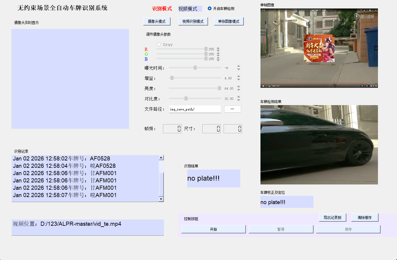
六、系统集成与GUI开发

• PyQt5界面设计
• 多线程处理
• 实时视频流处理
• 结果可视化

七、性能优化技巧

• 模型量化与压缩
• 推理速度优化
• 内存使用优化
• 多GPU并行处理

八、实际应用案例

• 停车场管理系统
• 交通违章检测
• 安防监控系统
• 移动端部署

九、常见问题与解决方案

• 光照条件变化
• 车牌倾斜变形
• 复杂背景干扰
• 低分辨率图像

十、未来发展方向

• 3D车牌识别
• 多模态融合
• 自监督学习
• 联邦学习应用

结语

本文详细介绍了基于深度学习的车牌识别系统的完整实现过程，从理论基础到代码实践，从模块设计到系统集成，为读者提供了全面的技术指导。车牌识别技术作为计算机视觉的重要应用，具有广阔的发展前景和实用价值。

通过本文的学习，读者可以：

1. 掌握深度学习在车牌识别中的应用
2. 理解YOLOv3、RetinaNet、LPRNet等先进算法
3. 具备完整的项目开发能力
4. 能够解决实际应用中的技术问题

希望本文能为您的学习和研究提供有价值的参考！

---