第一步--了解深度神经网络

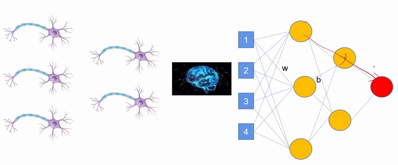
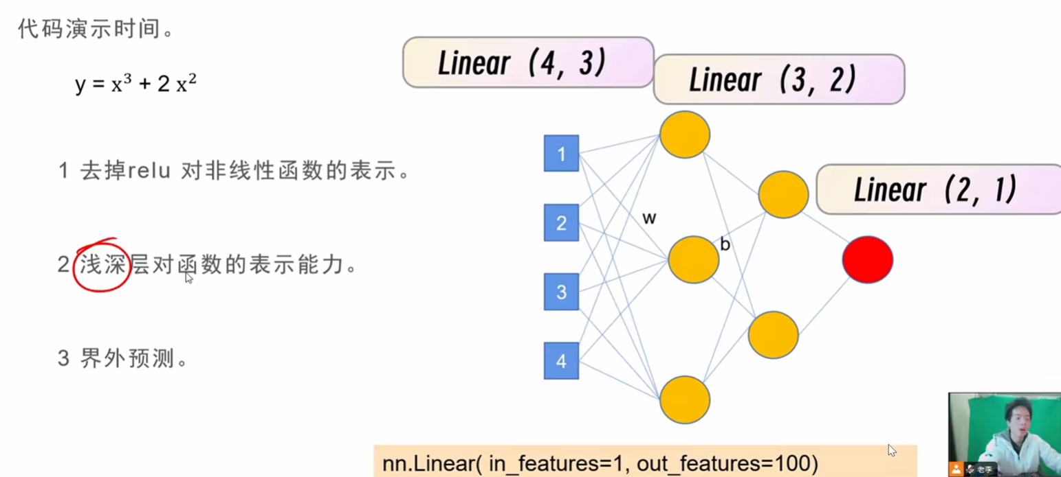
一、神经网络原理

1.神经元模型

本质上就是线性模型模拟神经元的功能， y=f(∑wx+b)

2.神经网络结构

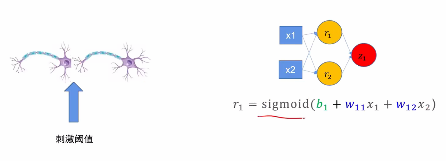
2.1神经元的串联

是通过类似于线性代数求和形式传递

不能只原封不动串联，那样没有任何意义，故而会有一个新的东西！

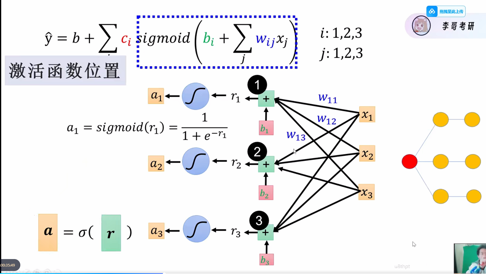
2.2激活函数！！

激活函数是非线性函数,有个很重要的特性：能求导

每一次传递会检测是否需要激活，如果没有达到要求不会传递到下一层

如果没有激活函数，就算层数再深，也变成了纯线性组合的输出，不能解决更加复杂的问题
经过激活函数，会对每一层的结果进行一个处理

有以下两个常见的激活函数

sigmoid函数

S(x)=11+e−x=exex+1 S(x) = \frac{1}{1 + e^{-x}} = \frac{e^x}{e^x + 1} S(x)=1+e−x1=ex+1ex

relu函数
f(x) = max(0,x)

激活函数就夹在这些 Layer 中间，故而激活函数一定要能求导

你可能会看到一个叫 ReLU 的激活函数，它长这样：f(x)=max⁡(0,x)f(x) = \max(0, x)f(x)=max(0,x)作为程序员，你一眼就会发现："等等！这个函数在 x=0 的那个折角处，也是不可导的啊！"没错，你的数学直觉很准。在 x=0x=0x=0 点，左导数是 0，右导数是 1，导数不连续。但是在深度学习的工程实践中，我们"作弊"了：我们在代码里强行规定：如果正好遇到 x=0x=0x=0，我们就把导数直接设为 0 或者 1（通常设为 0）。

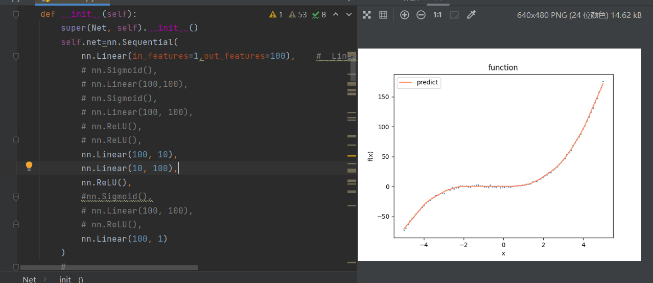
2.3加入激活函数的效果展示

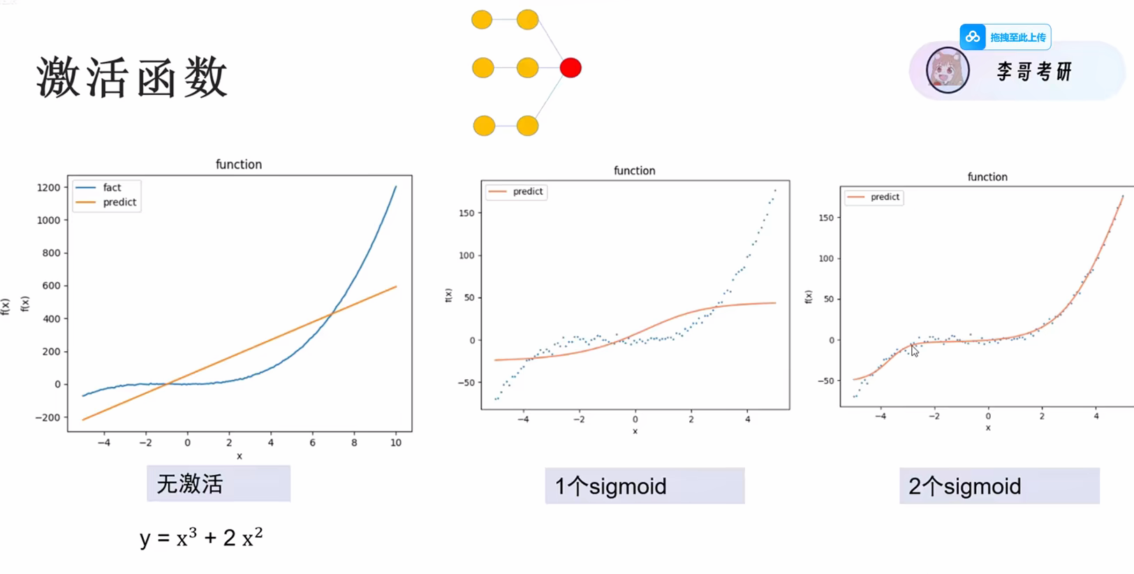
整体图形化表示

在这里插入图片描述

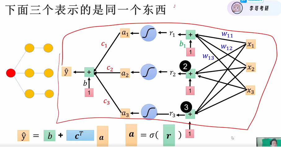
这时候我们再看看整体的模型结构（加上拟合和激活函数）

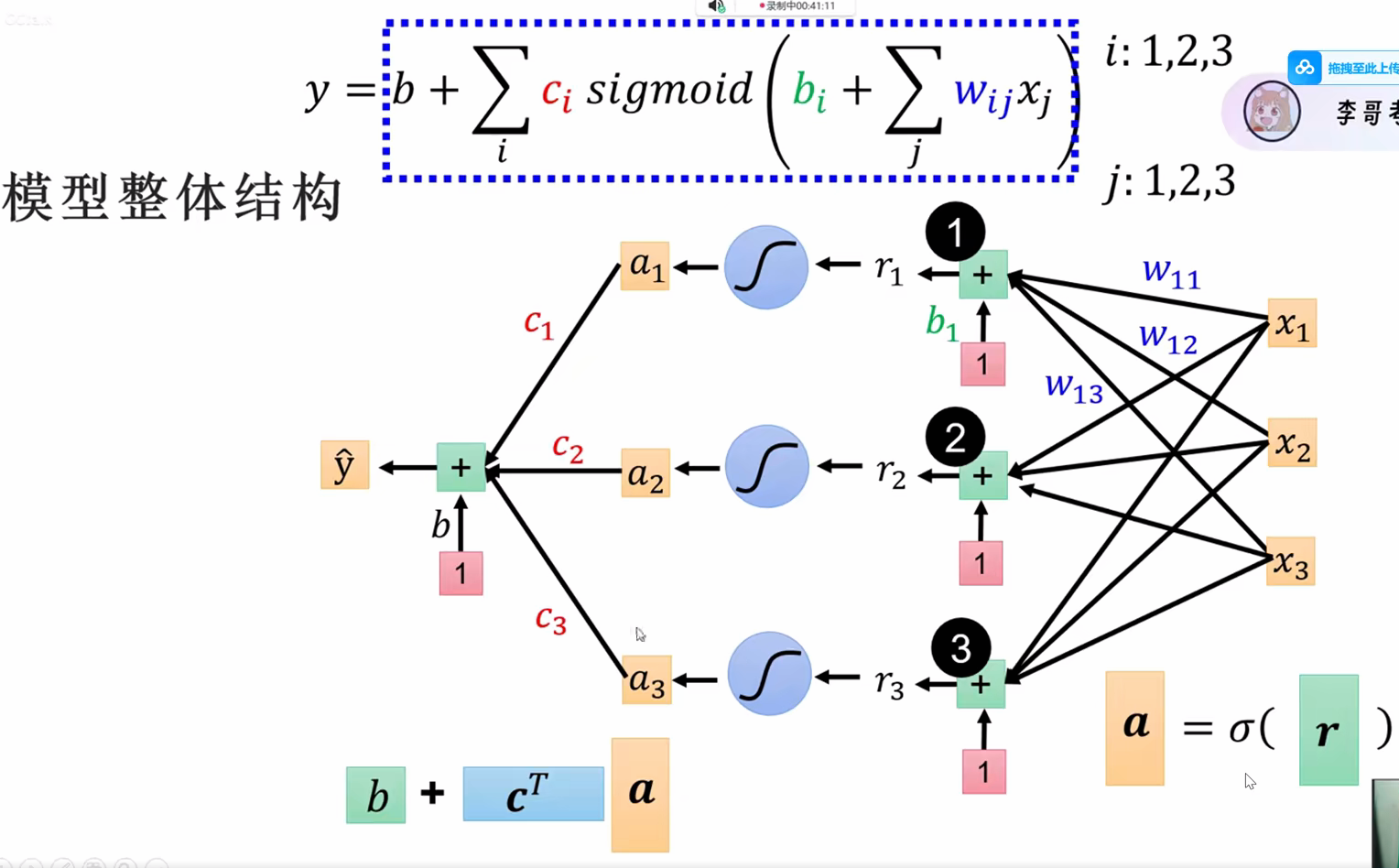
这样就可以让预测值不断地去接近实际值

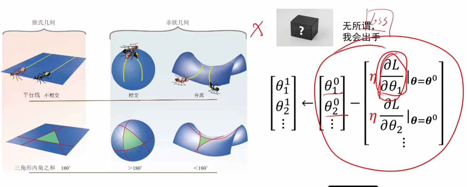
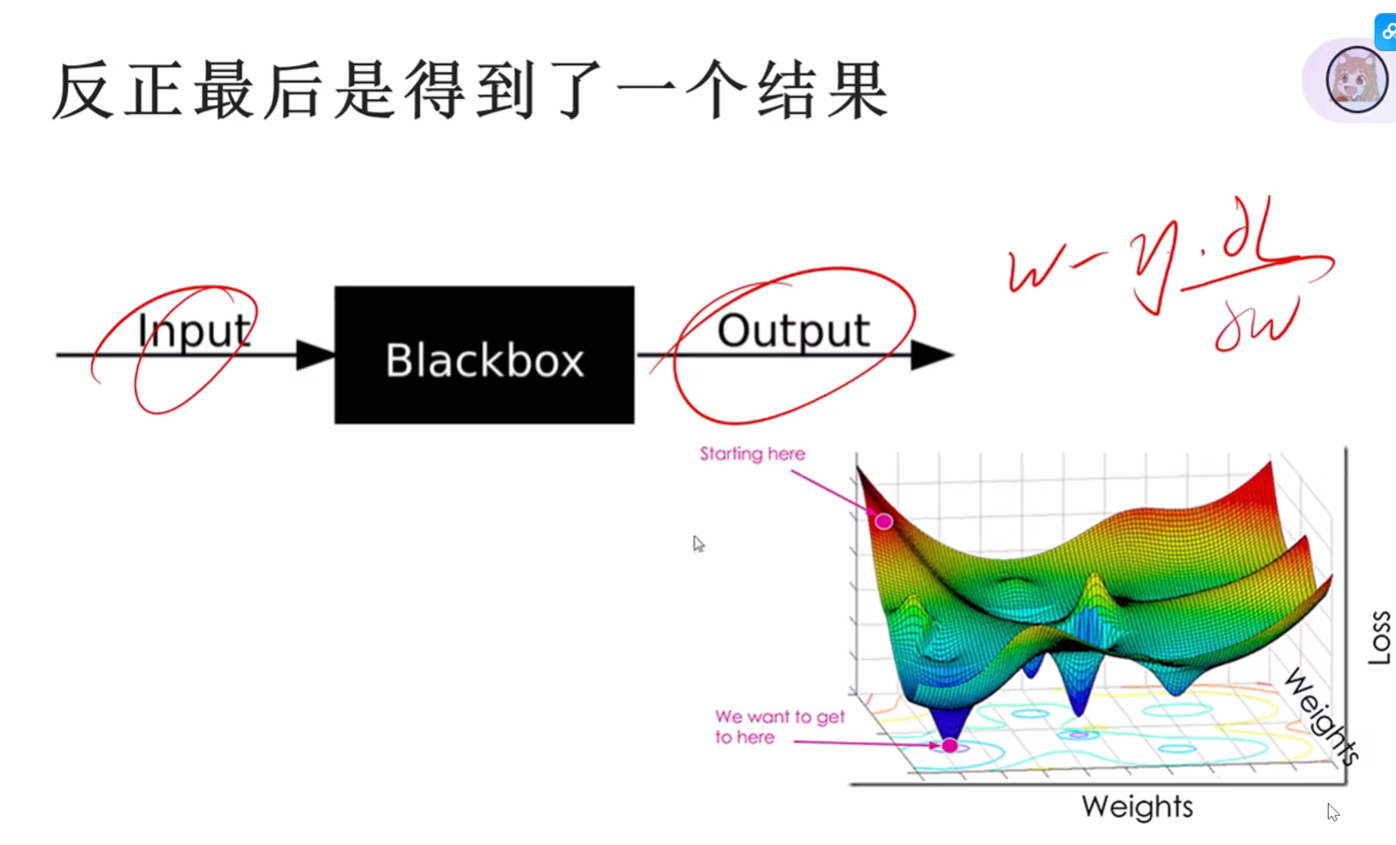
3.神经网络就是黑盒子

可能人为会去考虑如何生成的，但是在调参训练中，不断的降低loss的时候，实际上就是不断的计算梯度，不断的让w - 偏导的过程

这就是一个黑盒子，因为在我们看来整体就是在不断的求导，做减法

每一层都是全连接的网络

4.正式运行一个程序，理解激活函数的作用

python 复制代码

import random
import os
from torch.utils.data import DataLoader, Dataset
from torch.utils.data import TensorDataset
import torch.nn as nn
import numpy as np
import torch
import matplotlib.pyplot as plt

scatter = True


def seed_everything(seed):
    torch.manual_seed(seed)
    torch.cuda.manual_seed(seed)
    torch.cuda.manual_seed_all(seed)
    torch.backends.cudnn.benchmark = False
    torch.backends.cudnn.deterministic = True
    random.seed(seed)
    np.random.seed(seed)
    os.environ['PYTHONHASHSEED'] = str(seed)

seed_everything(0)     # 固定随机种子， 让我们每次运行都得到相同的结果。
#模型net
class Net(nn.Module):
    def __init__(self):
        super(Net, self).__init__()
        self.net=nn.Sequential(
            nn.Linear(in_features=1,out_features=100),    #  Linear model
            # nn.Sigmoid(),
            # nn.Linear(100,100),
            # nn.Sigmoid(),
            # nn.Linear(100, 100),
            # nn.ReLU(),
            # nn.ReLU(),
            nn.Linear(100, 10),
            nn.Linear(10, 100),
            #nn.ReLU(),
            nn.Sigmoid(),
            # nn.Linear(100, 100),
            # nn.ReLU(),
            nn.Linear(100, 1)
        )
        #
        #layer1 = nn.Linear(4,3)
        #layer2 = nn.Linear(3,2)
    def forward(self, input):
        return self.net(input)

class mydataset(Dataset):
    def __init__(self,x ,y):
        super(mydataset, self).__init__()
        self.x = torch.tensor(x,dtype=torch.float)
        self.y = torch.tensor(y,dtype=torch.float)

    def __getitem__(self, item):
        return self.x[item], self.y[item]

    def __len__(self):
        return len(self.x)


data_num = 100
# 准备数据
train_s = -5
train_e = 5
x=np.linspace(train_s,train_e, data_num)
# y=np.sin(x)

# y = 20*x+4
#创建数据

y = x**3 + 2*x**2 #模拟的函数


# 在输入上加入噪声。
mu = 0
sigma = 1
y += np.random.normal(mu, sigma, y.shape)
# for i in range(data_num):
#     y[i] += random.gauss(mu, sigma)

# 将数据做成数据集的模样
X=np.expand_dims(x,axis=1)
Y=y.reshape(data_num,-1)


# 使用批训练方式
# dataset=TensorDataset(torch.tensor(X,dtype=torch.float),torch.tensor(Y,dtype=torch.float))
dataset = mydataset(X, Y)
dataloader=DataLoader(dataset,batch_size=100,shuffle=True)


# 神经网络主要结构，这里就是一个简单的线性结构


net = Net()
# 定义优化器和损失函数
optim=torch.optim.Adam(net.parameters(net),lr=0.001)
# optim = torch.optim.SGD(net.parameters(), lr=0.01, momentum=0.09)
Loss = nn.MSELoss()



# 下面开始训练：
# 一共训练1000次
for epoch in range(1000):
    loss = None
    for batch_x,batch_y in dataloader:
        y_predict=net(batch_x)
        loss=Loss(y_predict,batch_y)
        optim.zero_grad()
        loss.backward()
        optim.step()

    # 每100次 的时候打印一次日志
    if (epoch+1)%100==0:
        print("step: {0} , loss: {1}".format(epoch+1,loss.item()))
        # 使用训练好的模型进行预测
        predict=net(torch.tensor(X,dtype=torch.float))
        # 绘图展示预测的和真实数据之间的差异
        if scatter:
            plt.scatter(x, y, 1)
        else:
            plt.plot(x,y,color="coral",label="fact")
        plt.plot(x,predict.detach().numpy(), color="coral",label="predict")
        plt.title("function")
        plt.xlabel("x")
        plt.ylabel("f(x)")
        plt.legend()
        # plt.savefig(fname="result.png",figsize=[10,10])
        plt.show()



# # 做一个测试集，解除注释可查看测试集结果
# if scatter:
#     plt.scatter(x,y,1)
# else:
#     plt.plot(x, y, label="fact")
#
# test_s = train_e
# test_e = test_s+5
# test_x = np.linspace(test_s, test_e, data_num)
# # y=np.sin(x)
# # y = 20*x+4
# test_y = test_x ** 3 + 2 * test_x ** 2

# # 将数据做成数据集的模样
# test_X = np.expand_dims(test_x, axis=1)
# test_Y = test_y.reshape(data_num, -1)
# # 使用批训练方式
# # test_dataset = TensorDataset(torch.tensor(test_X, dtype=torch.float), torch.tensor(test_Y, dtype=torch.float))
# # test_dataloader = DataLoader(test_dataset, batch_size=100, shuffle=True)
#
# pre = net(torch.tensor(test_X,dtype=torch.float))
#
#
#
# x = np.concatenate((x, test_x), axis=0)
# y = np.concatenate((y, test_y), axis=0)
#
# pre_y = np.concatenate((predict.detach().numpy(), pre.detach().numpy()), axis=0)
# plt.plot(x, pre_y, color="coral", label="predict")
#
# if scatter:
#     plt.scatter(x, y, 1,color="blue", label="fact")
# else:
#     plt.plot(x, y, label="fact",color="blue")
#
#
#
#
# # plt.title("sin function")
# plt.xlabel("x")
# plt.legend()
# # plt.savefig(fname="result.png",figsize=[10,10])
# plt.show()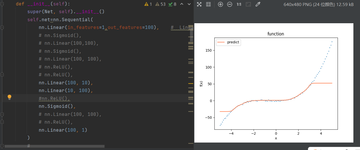

当把这里的sigmoid()换成ReLU()

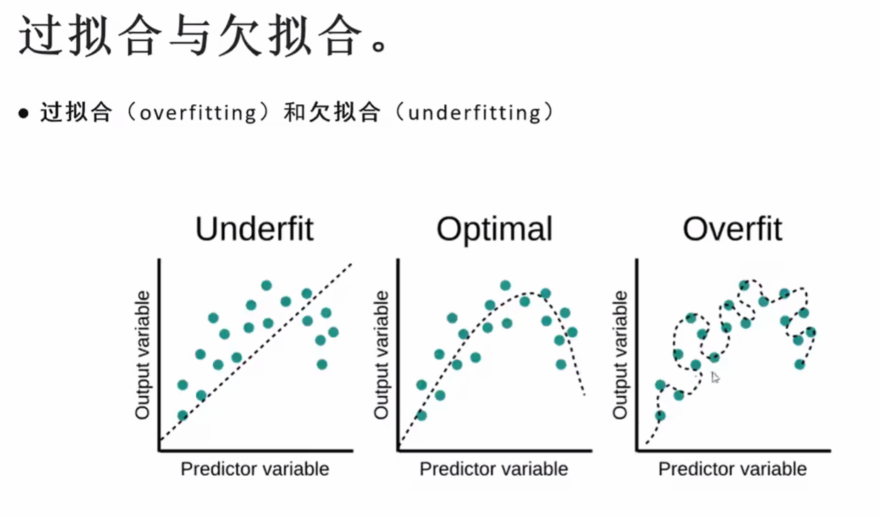
5.过拟合（overfit）和欠拟合(underfit)

上文中已经尝试了自己去调试模型的数据，输出的图像和训练集，看

看离真正的数据图像差距多远，在这个过程中，有两种状态，

如果模型够深的话，极有可能会变成过拟合

6.神经网络透析

函数的结构 = 模型的架构，神经网络本质上是架构设计。
神经网络在训练集上展现好没有用，在验证集上效果好才有用，偏偏神经网络在图片生成，人脸识别上，实现很不错，但是回归到原始的简单问题上，表现可能没有那么好，比如（模拟函数，判断一个数字是否偶数，发现数字规律）