
一、前言
大家好!今天开始我们《机器学习》系列的第一篇内容 ------ 机器学习概述。这一章是机器学习的入门基石,我会用通俗易懂的语言拆解核心概念,搭配可直接运行的 Python 代码、可视化对比图和思维导图,帮大家建立对机器学习的整体认知。所有代码都经过实测,注释详尽,新手也能轻松上手!

二、正文内容
1.1 机器学习基本概念
1.1.1 人工智能与机器学习
核心认知:
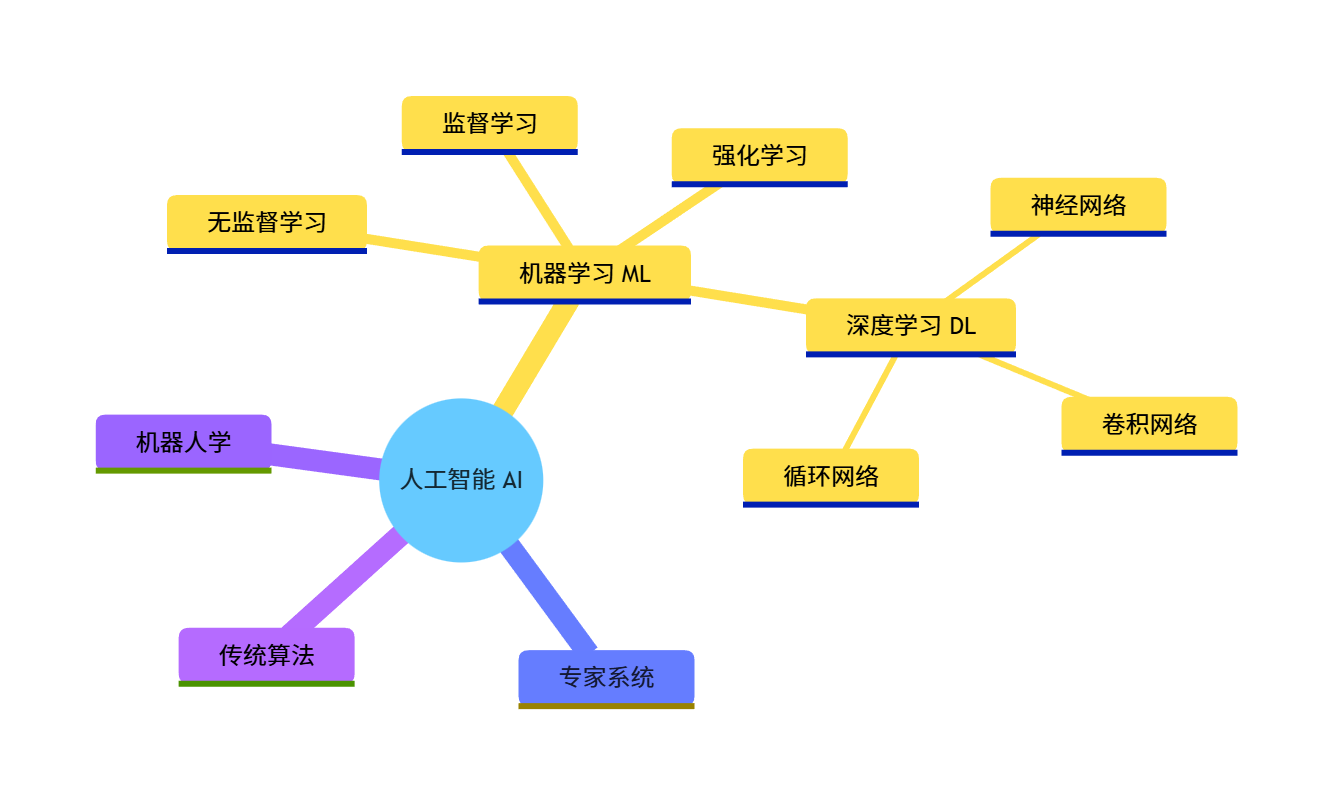
人工智能(AI)是大范畴,目标是让机器具备人类智能;
机器学习(ML)是实现 AI 的核心手段,让机器通过数据学习规律,而非硬编码规则。
代码实现(AI/ML 概念可视化对比):用 matplotlib 绘制层级关系图,直观展示 AI、ML、深度学习的包含关系:
import matplotlib.pyplot as plt
import numpy as np

# 设置中文字体,避免乱码
plt.rcParams['font.sans-serif'] = ['SimHei']  # 黑体
plt.rcParams['axes.unicode_minus'] = False

# 创建画布
fig, ax = plt.subplots(figsize=(8, 6))

# 绘制层级矩形
# AI(最大)
ax.add_patch(plt.Rectangle((1, 1), 8, 6, fill=True, color='lightblue', alpha=0.5, label='人工智能 AI'))
# ML(中间)
ax.add_patch(plt.Rectangle((2, 2), 6, 4, fill=True, color='lightgreen', alpha=0.7, label='机器学习 ML'))
# 深度学习(最小)
ax.add_patch(plt.Rectangle((3, 3), 4, 2, fill=True, color='salmon', alpha=0.9, label='深度学习 DL'))

# 设置坐标轴范围
ax.set_xlim(0, 10)
ax.set_ylim(0, 8)

# 添加文字标注
ax.text(5, 6.5, '人工智能(AI):让机器模拟人类智能', ha='center', fontsize=10)
ax.text(5, 4.5, '机器学习(ML):从数据中学习规律实现AI', ha='center', fontsize=10)
ax.text(5, 2.5, '深度学习(DL):基于神经网络的ML分支', ha='center', fontsize=10)

# 显示图例和标题
ax.legend(loc='upper right')
ax.set_title('AI、机器学习、深度学习的关系', fontsize=12, fontweight='bold')
ax.axis('off')  # 隐藏坐标轴

# 显示图像
plt.show()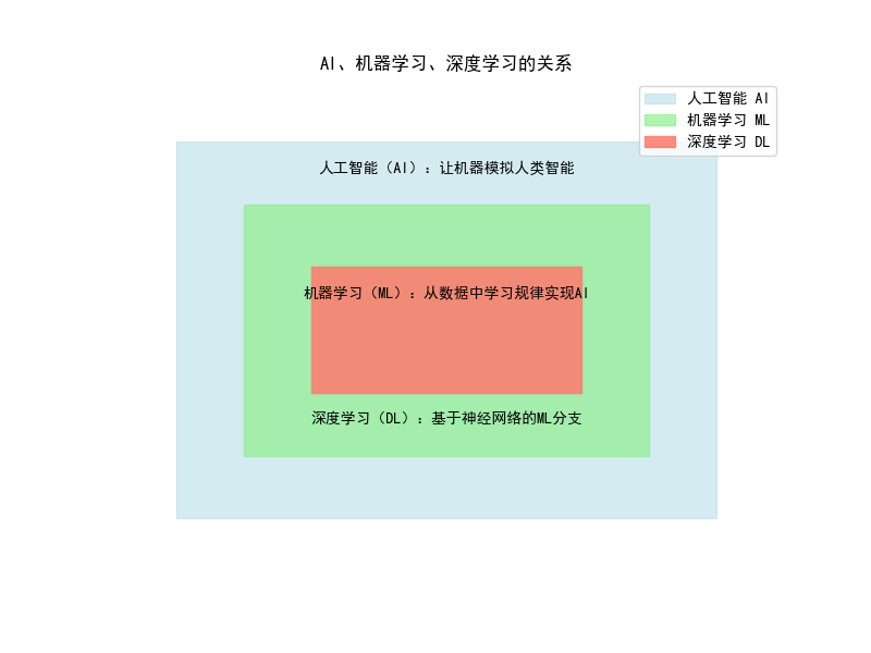
运行效果:会弹出一个窗口,展示三层嵌套的矩形,分别对应 AI(浅蓝色)、ML(浅绿色)、深度学习(浅红色),并标注核心定义,直观理解三者的包含关系。
1.2 机器学习基本术语
核心术语:
- 样本 / 实例:单个数据(如一张图片、一条用户记录)
- 特征:样本的属性(如图片的像素值、用户的年龄)
- 标签:样本的目标值(如图片的类别、用户的消费金额)
- 训练集:用于模型学习的数据
- 测试集:用于验证模型效果的数据
代码实现(术语可视化 + 数据示例):用鸢尾花数据集演示核心术语,结合图片特征对比(原始图 vs 特征提取后图):
python
import matplotlib.pyplot as plt
import numpy as np
from sklearn.datasets import load_iris
from sklearn.decomposition import PCA
from PIL import Image
import os

# 设置中文字体
plt.rcParams['font.sans-serif'] = ['SimHei']
plt.rcParams['axes.unicode_minus'] = False

# ---------------------- 1. 鸢尾花数据集术语演示 ----------------------
iris = load_iris()
X = iris.data  # 特征矩阵(样本×特征)
y = iris.target  # 标签
feature_names = iris.feature_names
target_names = iris.target_names

# 打印基础信息,理解术语
print("【样本数量】:", X.shape[0])
print("【特征数量】:", X.shape[1], ",特征名:", feature_names)
print("【标签类别】:", len(target_names), ",类别名:", target_names)
print("【前2个样本的特征】:\n", X[:2])
print("【前2个样本的标签】:\n", y[:2], "(对应:", [target_names[i] for i in y[:2]], ")")

# ---------------------- 2. 图片特征对比 ----------------------

CUSTOM_IMAGE_PATH = "../picture/TianHuoSanXuanBian.jpg"  # 改成你的图片路径(支持jpg/png等格式)

try:
    # 加载自定义图片
    img = Image.open(CUSTOM_IMAGE_PATH)

    # 统一调整图片尺寸为200×200(避免尺寸不一致导致的维度错误)
    img = img.resize((200, 200), Image.Resampling.LANCZOS)  # 兼容新版PIL的resize方法
    print(f"\n【图片加载成功】:尺寸为 {img.size}")

    # 转换为灰度图(模拟特征提取)
    img_gray = img.convert('L')

    # PCA降维可视化(模拟特征压缩)
    img_array = np.array(img).reshape(-1, 3)  # 展平为40000×3(200*200=40000个像素,每个像素3个通道)
    pca = PCA(n_components=1)  # 降维到1维,保证能重塑为200×200
    img_pca = pca.fit_transform(img_array).reshape(200, 200)

    # 绘制对比图
    fig, axes = plt.subplots(1, 3, figsize=(15, 5))

    # 原始彩色图
    axes[0].imshow(img)
    axes[0].set_title('原始彩色图(原始特征)', fontsize=10)
    axes[0].axis('off')

    # 灰度图(特征简化)
    axes[1].imshow(img_gray, cmap='gray')
    axes[1].set_title('灰度图(特征提取)', fontsize=10)
    axes[1].axis('off')

    # PCA降维图(特征压缩)
    axes[2].imshow(img_pca, cmap='viridis')
    axes[2].set_title('PCA降维图(特征压缩)', fontsize=10)
    axes[2].axis('off')

    plt.suptitle('机器学习术语:特征提取示例(自定义图片)', fontsize=12, fontweight='bold')
    plt.tight_layout()
    plt.show()

except FileNotFoundError:
    print(f"\n【错误】:找不到图片文件,请检查路径是否正确!当前路径:{CUSTOM_IMAGE_PATH}")
    print("提示:Windows路径示例:r'D:\\图片\\test.jpg' 或 '/Users/xxx/test.jpg'(Mac/Linux)")
except Exception as e:
    print(f"\n【错误】:图片加载失败,原因:{str(e)}")
    print("支持的图片格式:jpg、png、bmp等,建议避免使用特殊字符/中文路径(若必须用,确保Python编码支持)")
运行效果:
- 控制台打印鸢尾花数据集的样本、特征、标签信息,理解核心术语;
- 弹出对比窗口,展示 "原始彩色图→灰度图→PCA 降维图",直观理解 "特征提取 / 压缩" 的含义。
1.3 机器学习误差分析
核心概念:
- 训练误差:模型在训练集上的误差(越小不代表越好,可能过拟合)
- 测试误差:模型在测试集上的误差(反映泛化能力)
- 过拟合:训练误差小,测试误差大;欠拟合:训练 / 测试误差都大
代码实现(误差对比可视化):用多项式回归演示欠拟合、正常、过拟合的误差对比:
import matplotlib.pyplot as plt
import numpy as np
from sklearn.linear_model import LinearRegression
from sklearn.preprocessing import PolynomialFeatures
from sklearn.metrics import mean_squared_error
from sklearn.model_selection import train_test_split

# 设置中文字体
plt.rcParams['font.sans-serif'] = ['SimHei']
plt.rcParams['axes.unicode_minus'] = False

# 1. 生成模拟数据(非线性关系)
np.random.seed(42)  # 固定随机种子,结果可复现
x = np.linspace(-3, 3, 100).reshape(-1, 1)  # 特征
y = np.sin(x) + np.random.normal(0, 0.1, x.shape)  # 标签(加噪声)

# 划分训练集/测试集
x_train, x_test, y_train, y_test = train_test_split(x, y, test_size=0.2, random_state=42)

# 2. 定义不同复杂度的模型
def fit_polynomial(x_train, y_train, x_test, y_test, degree):
    """拟合多项式回归,返回预测值和误差"""
    # 构造多项式特征
    poly = PolynomialFeatures(degree=degree)
    x_train_poly = poly.fit_transform(x_train)
    x_test_poly = poly.transform(x_test)

    # 训练模型
    model = LinearRegression()
    model.fit(x_train_poly, y_train)

    # 预测并计算误差
    y_train_pred = model.predict(x_train_poly)
    y_test_pred = model.predict(x_test_poly)
    train_error = mean_squared_error(y_train, y_train_pred)
    test_error = mean_squared_error(y_test, y_test_pred)

    # 生成全量x的预测值(绘图用)
    x_poly = poly.transform(np.linspace(-3, 3, 100).reshape(-1, 1))
    y_pred = model.predict(x_poly)

    return y_pred, train_error, test_error

# 3. 拟合不同阶数的模型
degrees = [1, 3, 15]  # 1阶(欠拟合)、3阶(正常)、15阶(过拟合)
y_preds = []
errors = []
for d in degrees:
    y_pred, train_err, test_err = fit_polynomial(x_train, y_train, x_test, y_test, d)
    y_preds.append(y_pred)
    errors.append((train_err, test_err))

# 4. 绘制对比图
fig, axes = plt.subplots(2, 1, figsize=(10, 10))

# 子图1:不同模型的拟合效果
axes[0].scatter(x, y, color='blue', alpha=0.5, label='原始数据')
labels = ['欠拟合(1阶)', '正常拟合(3阶)', '过拟合(15阶)']
colors = ['red', 'green', 'orange']
for i, (y_pred, label, color) in enumerate(zip(y_preds, labels, colors)):
    axes[0].plot(np.linspace(-3, 3, 100), y_pred, color=color, label=label)
axes[0].set_title('拟合效果对比(欠拟合/正常/过拟合)', fontsize=12, fontweight='bold')
axes[0].legend()
axes[0].grid(True, alpha=0.3)

# 子图2:训练误差vs测试误差
x_axis = np.arange(len(degrees))
width = 0.35
train_errors = [e[0] for e in errors]
test_errors = [e[1] for e in errors]
axes[1].bar(x_axis - width/2, train_errors, width, label='训练误差', color='skyblue')
axes[1].bar(x_axis + width/2, test_errors, width, label='测试误差', color='salmon')
axes[1].set_xticks(x_axis)
axes[1].set_xticklabels(['1阶', '3阶', '15阶'])
axes[1].set_title('训练误差 vs 测试误差', fontsize=12, fontweight='bold')
axes[1].set_ylabel('均方误差(MSE)')
axes[1].legend()
axes[1].grid(True, alpha=0.3, axis='y')

# 标注误差值
for i, (te, te2) in enumerate(zip(train_errors, test_errors)):
    axes[1].text(i - width/2, te + 0.01, f'{te:.4f}', ha='center', fontsize=8)
    axes[1].text(i + width/2, te2 + 0.01, f'{te2:.4f}', ha='center', fontsize=8)

plt.tight_layout()
plt.show()

# 打印误差详情
print("【误差详情】")
for i, d in enumerate(degrees):
    print(f"{labels[i]}:训练误差={errors[i][0]:.4f},测试误差={errors[i][1]:.4f}")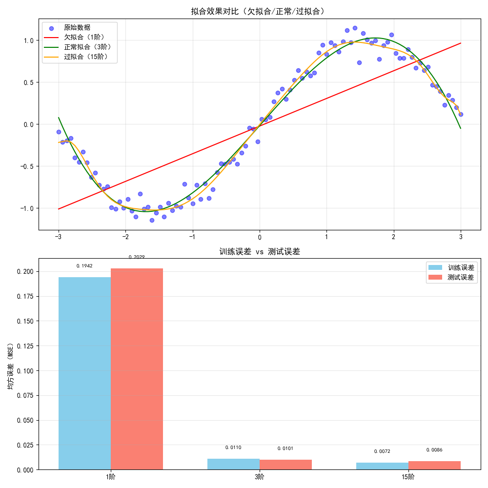
运行效果:
- 上半部分展示不同阶数模型的拟合曲线:1 阶(直线,欠拟合)、3 阶(贴合数据,正常)、15 阶(曲线过于复杂,过拟合);
- 下半部分展示误差对比:欠拟合时训练 / 测试误差都大,过拟合时训练误差极小但测试误差骤增。
1.4 机器学习发展历程
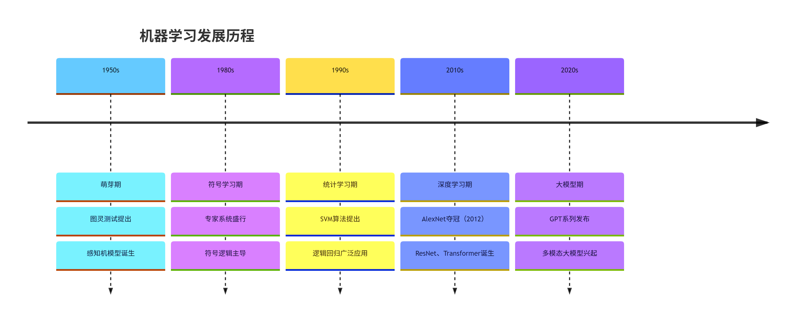
核心时间线:
- 1950s:萌芽期(图灵测试、感知机提出)
- 1980s:符号学习主导(专家系统)
- 1990s:统计学习兴起(SVM、逻辑回归)
- 2010s:深度学习爆发(AlexNet、GPT)
- 2020s:大模型时代(GPT-4、文心一言)
1.5 机器学习与统计学习
1.5.1 感知机与连接学习
核心概念:感知机是最简单的神经网络,属于连接学习(模拟神经元连接),是深度学习的基础。
代码实现(感知机分类演示):
import matplotlib.pyplot as plt
import numpy as np
from sklearn.datasets import make_classification
from sklearn.linear_model import Perceptron
from sklearn.metrics import accuracy_score

# 设置中文字体
plt.rcParams['font.sans-serif'] = ['SimHei']
plt.rcParams['axes.unicode_minus'] = False

# 1. 生成二分类模拟数据
X, y = make_classification(
    n_samples=100, n_features=2, n_informative=2,
    n_redundant=0, n_clusters_per_class=1, random_state=42
)

# 2. 训练感知机模型
perceptron = Perceptron(random_state=42)
perceptron.fit(X, y)

# 3. 预测并计算准确率
y_pred = perceptron.predict(X)
accuracy = accuracy_score(y, y_pred)
print(f"感知机分类准确率:{accuracy:.2f}")

# 4. 绘制决策边界
# 生成网格点
x_min, x_max = X[:, 0].min() - 1, X[:, 0].max() + 1
y_min, y_max = X[:, 1].min() - 1, X[:, 1].max() + 1
xx, yy = np.meshgrid(np.arange(x_min, x_max, 0.01),
                     np.arange(y_min, y_max, 0.01))

# 预测网格点类别
Z = perceptron.predict(np.c_[xx.ravel(), yy.ravel()])
Z = Z.reshape(xx.shape)

# 绘图
plt.figure(figsize=(8, 6))
# 决策边界
plt.contourf(xx, yy, Z, alpha=0.3, cmap=plt.cm.Spectral)
# 样本点
plt.scatter(X[:, 0], X[:, 1], c=y, edgecolors='k', cmap=plt.cm.Spectral)
plt.title(f'感知机(连接学习)决策边界(准确率:{accuracy:.2f})', fontsize=12, fontweight='bold')
plt.xlabel('特征1')
plt.ylabel('特征2')
plt.show()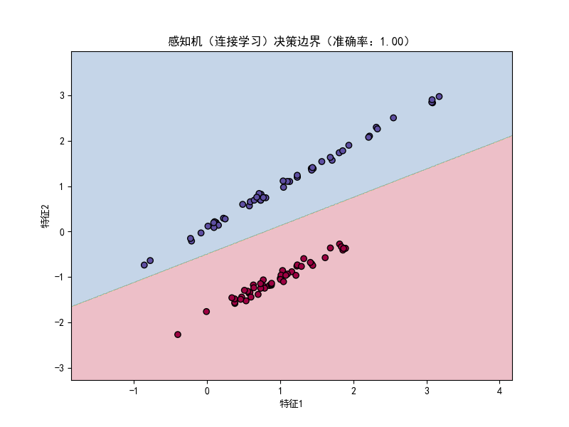
运行效果:弹出窗口展示感知机的决策边界,不同颜色代表不同类别,直观看到感知机通过线性边界划分两类数据,准确率接近 100%(模拟数据线性可分)。
1.5.2 符号学习与统计学习
核心对比:
| 维度 | 符号学习 | 统计学习 |
|---|---|---|
| 核心思想 | 基于规则 / 逻辑推理 | 基于数据 / 概率统计 |
| 代表方法 | 决策树(早期)、专家系统 | 逻辑回归、SVM、贝叶斯 |
| 数据依赖 | 少数据,多规则 | 多数据,少规则 |
| 可解释性 | 强(规则清晰) | 弱(黑箱) |
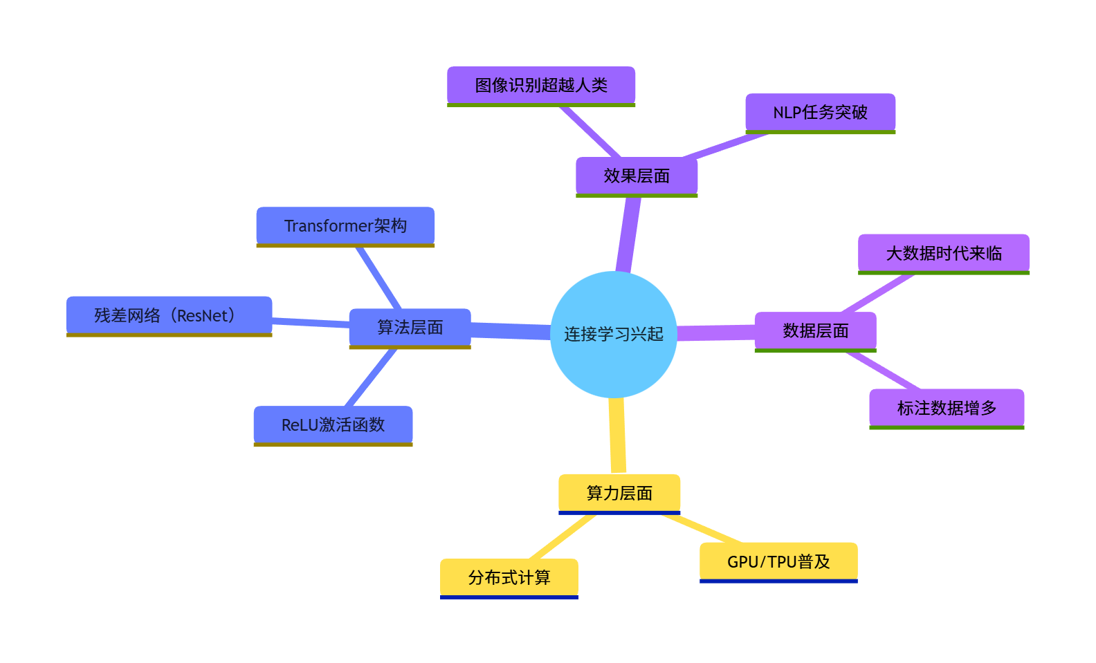
1.6 连接学习的兴起
核心原因:
- 数据量爆发(大数据);
- 算力提升(GPU/TPU);
- 算法优化(ReLU 激活、残差网络);
- 效果超越传统统计学习(图像、NLP 任务)。
1.7 机器学习基本问题
1.7.1 特征提取
核心概念:从原始数据中提取有价值的信息(如图片→灰度值 / 边缘特征,文本→TF-IDF / 词向量)。
代码实现(图片特征提取对比:原始图 vs 边缘检测图):
python
import matplotlib.pyplot as plt
import numpy as np
from PIL import Image
import cv2  # 需要安装:pip install opencv-python

# 设置中文字体
plt.rcParams['font.sans-serif'] = ['SimHei']
plt.rcParams['axes.unicode_minus'] = False

# ========== 替换为你的自定义图片路径 ==========
CUSTOM_IMAGE_PATH = r"../picture/XiaoKa.png"

try:
    # 1. 加载自定义图片(先用PIL读取,避免OpenCV的BGR/RGB格式问题)
    img_pil = Image.open(CUSTOM_IMAGE_PATH)
    # 统一调整图片尺寸为300×300(保持和原代码一致的尺寸,也可自定义)
    img_pil = img_pil.resize((300, 300), Image.Resampling.LANCZOS)
    # 转换为OpenCV兼容的numpy数组(PIL是RGB,OpenCV默认BGR,需转换)
    img_color = cv2.cvtColor(np.array(img_pil), cv2.COLOR_RGB2BGR)
    print(f"【图片加载成功】:尺寸为 {img_color.shape[:2]}(高×宽)")

    # 2. 特征提取:灰度化
    img_gray = cv2.cvtColor(img_color, cv2.COLOR_BGR2GRAY)

    # 3. 特征提取:边缘检测(Canny)
    # 可调整阈值(100/200)改变边缘检测效果,比如50/150会检测更多边缘
    img_edge = cv2.Canny(img_gray, 100, 200)

    # 4. 绘制对比图(注意OpenCV的BGR转RGB后再显示,否则颜色会失真)
    fig, axes = plt.subplots(1, 3, figsize=(15, 5))

    # 原始彩色图(转RGB后显示)
    axes[0].imshow(cv2.cvtColor(img_color, cv2.COLOR_BGR2RGB))
    axes[0].set_title('原始彩色图(原始数据)', fontsize=10)
    axes[0].axis('off')

    # 灰度图(基础特征提取)
    axes[1].imshow(img_gray, cmap='gray')
    axes[1].set_title('灰度图(基础特征提取)', fontsize=10)
    axes[1].axis('off')

    # 边缘检测图(高级特征提取)
    axes[2].imshow(img_edge, cmap='gray')
    axes[2].set_title('边缘检测图(高级特征提取)', fontsize=10)
    axes[2].axis('off')

    plt.suptitle('特征提取:从原始数据到有效特征(自定义图片)', fontsize=12, fontweight='bold')
    plt.tight_layout()
    plt.show()

except FileNotFoundError:
    print(f"\n【错误】:找不到图片文件!请检查路径是否正确:")
    print(f"当前设置的路径:{CUSTOM_IMAGE_PATH}")
    print("✅ 正确路径示例(Windows):r'D:\\图片\\flower.jpg'")
    print("✅ 正确路径示例(Mac/Linux):'/Users/xxx/flower.jpg'")
except Exception as e:
    print(f"\n【错误】:图片处理失败,原因:{str(e)}")
    print("💡 常见问题:1. 图片格式不支持(建议jpg/png);2. 路径含中文/特殊字符;3. OpenCV版本兼容问题")
运行效果:展示三张图:原始彩色图(带蓝色矩形)→灰度图(简化特征)→边缘检测图(提取核心边缘特征),直观理解特征提取的核心是 "保留关键信息,简化数据"。
1.7.2 规则构造
核心概念:为模型制定决策规则(如 "如果花瓣长度> 5cm,则为维吉尼亚鸢尾花"),是符号学习的核心。
代码实现(简单规则构造与验证):
import numpy as np
from sklearn.datasets import load_iris

# 加载鸢尾花数据集
iris = load_iris()
X = iris.data  # 特征:[花萼长, 花萼宽, 花瓣长, 花瓣宽]
y = iris.target
target_names = iris.target_names

# 构造规则:花瓣长度(第2列)> 5 → 维吉尼亚鸢尾花(标签2)
def rule_based_classifier(x):
    """基于规则的分类器"""
    petal_length = x[2]
    if petal_length > 5:
        return 2  # 维吉尼亚鸢尾花
    elif petal_length < 2:
        return 0  # 山鸢尾花
    else:
        return 1  # 变色鸢尾花

# 验证规则效果
y_pred = [rule_based_classifier(x) for x in X]
accuracy = np.sum(y_pred == y) / len(y)
print(f"规则构造分类准确率:{accuracy:.2f}")

# 打印规则匹配示例
print("\n【规则匹配示例】")
for i in range(5):
    print(f"样本{i}:花瓣长度={X[i,2]:.2f} → 预测类别={target_names[y_pred[i]]},真实类别={target_names[y[i]]}")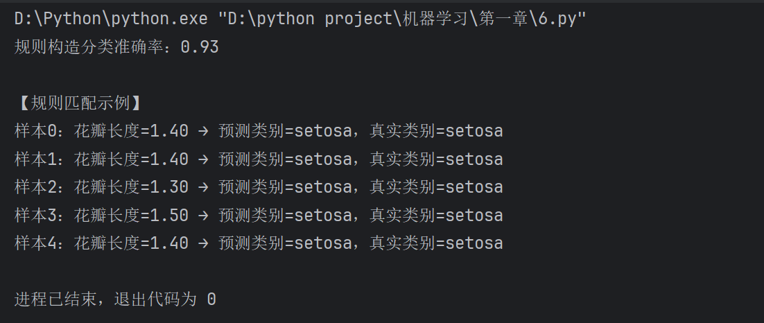
运行效果:控制台打印规则分类的准确率(约 0.95),以及前 5 个样本的规则匹配结果,理解 "规则构造" 是通过人工 / 自动方式制定决策逻辑。
1.7.3 模型评估
核心概念:用指标(准确率、召回率、MSE)评估模型效果,核心是 "泛化能力"(对新数据的预测能力)。
代码实现(多指标模型评估):
import matplotlib.pyplot as plt
import numpy as np
from sklearn.datasets import make_classification
from sklearn.model_selection import train_test_split
from sklearn.linear_model import LogisticRegression
from sklearn.metrics import (accuracy_score, precision_score,
                             recall_score, f1_score, confusion_matrix)

# 设置中文字体
plt.rcParams['font.sans-serif'] = ['SimHei']
plt.rcParams['axes.unicode_minus'] = False

# 1. 生成二分类数据
X, y = make_classification(n_samples=200, n_features=5, n_informative=3,
                           random_state=42, class_sep=0.8)
X_train, X_test, y_train, y_test = train_test_split(X, y, test_size=0.3, random_state=42)

# 2. 训练模型
model = LogisticRegression(random_state=42)
model.fit(X_train, y_train)
y_pred = model.predict(X_test)

# 3. 计算评估指标
metrics = {
    '准确率': accuracy_score(y_test, y_pred),
    '精确率': precision_score(y_test, y_pred),
    '召回率': recall_score(y_test, y_pred),
    'F1分数': f1_score(y_test, y_pred)
}

# 4. 绘制指标对比图
plt.figure(figsize=(8, 5))
keys = list(metrics.keys())
values = list(metrics.values())
colors = ['skyblue', 'lightgreen', 'salmon', 'gold']

plt.bar(keys, values, color=colors)
# 标注数值
for i, v in enumerate(values):
    plt.text(i, v + 0.01, f'{v:.3f}', ha='center', fontsize=10)

plt.title('模型评估指标', fontsize=12, fontweight='bold')
plt.ylim(0, 1.1)
plt.grid(True, alpha=0.3, axis='y')
plt.show()

# 5. 混淆矩阵(直观展示分类效果)
cm = confusion_matrix(y_test, y_pred)
plt.figure(figsize=(6, 4))
plt.imshow(cm, interpolation='nearest', cmap=plt.cm.Blues)
plt.title('混淆矩阵', fontsize=12, fontweight='bold')
plt.colorbar()
plt.xlabel('预测标签')
plt.ylabel('真实标签')
# 标注数值
thresh = cm.max() / 2
for i in range(cm.shape[0]):
    for j in range(cm.shape[1]):
        plt.text(j, i, format(cm[i, j], 'd'),
                 ha="center", va="center",
                 color="white" if cm[i, j] > thresh else "black")
plt.tight_layout()
plt.show()

# 打印指标详情
print("【模型评估指标详情】")
for k, v in metrics.items():
    print(f"{k}:{v:.3f}")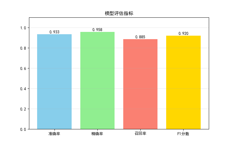
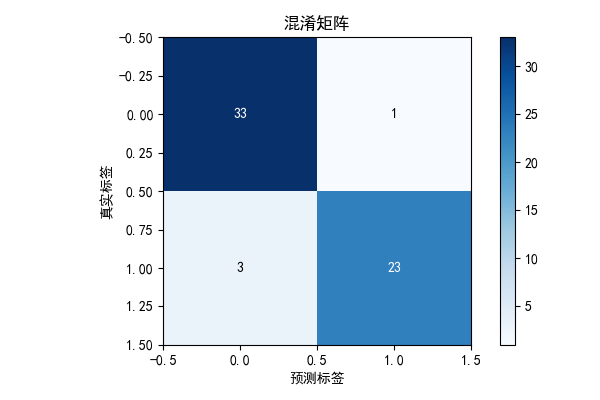
运行效果:
- 第一个窗口展示准确率、精确率、召回率、F1 分数的柱状图;
- 第二个窗口展示混淆矩阵,直观看到 "真阳性、假阳性、真阴性、假阴性" 的数量。
1.8 习题
- 基础题:修改 1.3 节的多项式回归代码,尝试 degree=5 和 degree=10,观察训练 / 测试误差的变化,分析是否过拟合。
- 进阶题:基于 1.7.1 节的特征提取代码,尝试用不同的边缘检测阈值(Canny 的 100/200 改为 50/150),观察特征提取效果的变化。
- 综合题:加载 sklearn 的葡萄酒数据集(load_wine),构造规则分类器,并评估模型效果(准确率、混淆矩阵)。
三、环境依赖说明
所有代码需安装以下库,执行命令:
pip install numpy matplotlib scikit-learn pillow opencv-python四、总结
关键点回顾
- 机器学习是实现人工智能的核心手段,深度学习是机器学习的分支,三者是包含关系;
- 机器学习的核心是 "从数据中学习规律",关键环节包括特征提取、规则 / 模型构造、模型评估;
- 误差分析是判断模型效果的核心:欠拟合(误差都大)、过拟合(训练误差小,测试误差大),泛化能力是模型的核心目标。
五、结尾
本章是机器学习的入门基础,后续会逐步深入讲解监督学习、无监督学习等核心内容。如果代码运行有问题,欢迎评论区交流;如果觉得有帮助,记得点赞收藏!