图像的卷积操作

卷积操作是一种线性滤波技术，通过在图像上滑动一个卷积核（滤波器）来提取图像特征。每个输出像素是卷积核与对应图像区域像素的加权和。

卷积操作步骤：

滑动卷积核：在图像上逐像素移动卷积核
对应相乘：卷积核权重与图像对应像素值相乘
求和：将所有乘积相加得到输出像素值
边缘处理：通常需要对图像边缘进行填充（如补0）
见卷积核类型：
边缘检测：Sobel, Laplacian, Prewitt
模糊/平滑：平均模糊，高斯模糊
锐化：增强边缘对比度

浮雕：创建3D效果

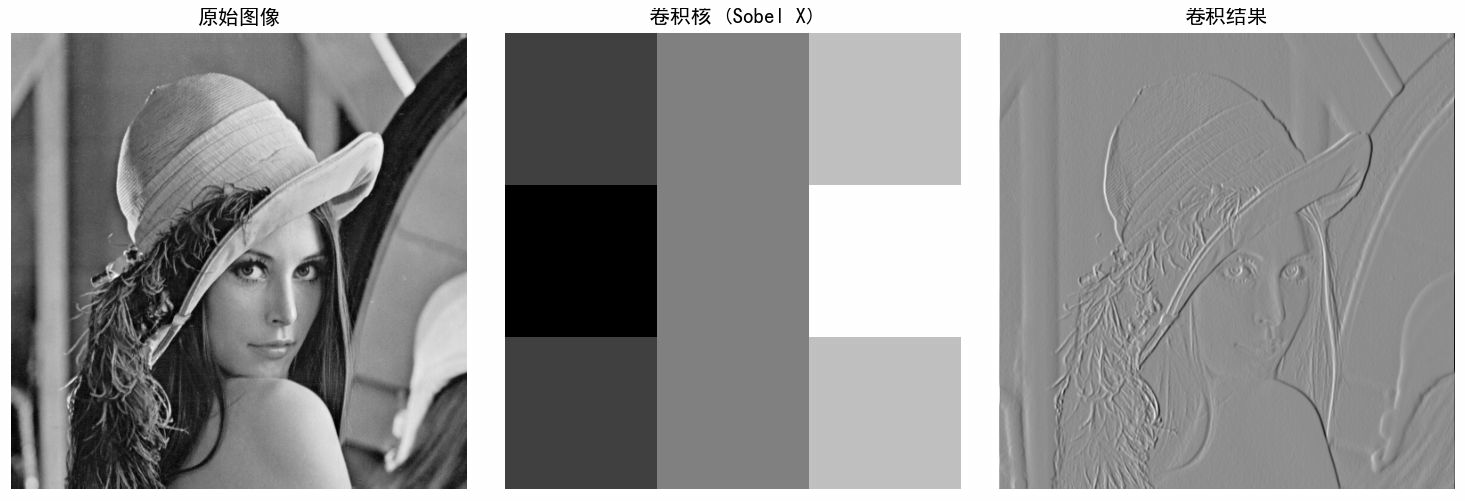
python 复制代码

# ====================
# 1. 基础卷积实现
# ====================

def conv2d(image, kernel, padding=0, stride=1):
	"""
	2D卷积实现
	:param image: 输入图像（2D数组）
	:param kernel: 卷积核（2D数组）
	:param padding: 边缘填充大小
	:param stride: 步长
	:return: 卷积结果
	"""
	# 添加padding
	if padding > 0:
		image = np.pad(image, padding, mode='constant')

	# 获取尺寸
	img_h, img_w = image.shape
	kernel_h, kernel_w = kernel.shape

	# 计算输出尺寸
	output_h = (img_h - kernel_h) // stride + 1
	output_w = (img_w - kernel_w) // stride + 1

	# 初始化输出
	output = np.zeros((output_h, output_w))

	# 卷积计算
	for y in range(0, output_h):
		for x in range(0, output_w):
			# 计算当前区域
			y_start = y * stride
			y_end = y_start + kernel_h
			x_start = x * stride
			x_end = x_start + kernel_w

			# 提取图像区域
			region = image[y_start:y_end, x_start:x_end]

			# 卷积计算
			output[y, x] = np.sum(region * kernel)

	return output


# ====================
# 2. 常见卷积核示例
# ====================

# 定义常用卷积核
kernels = {
	# 边缘检测
	'sobel_x': np.array([[-1, 0, 1],
	                     [-2, 0, 2],
	                     [-1, 0, 1]]),

	'sobel_y': np.array([[-1, -2, -1],
	                     [0, 0, 0],
	                     [1, 2, 1]]),

	'laplacian': np.array([[0, 1, 0],
	                       [1, -4, 1],
	                       [0, 1, 0]]),

	# 模糊/平滑
	'box_blur': np.ones((3, 3)) / 9,

	'gaussian_blur': np.array([[1, 2, 1],
	                           [2, 4, 2],
	                           [1, 2, 1]]) / 16,

	# 锐化
	'sharpen': np.array([[0, -1, 0],
	                     [-1, 5, -1],
	                     [0, -1, 0]])
}
# ====================
	# 6. 多通道图像卷积
	# ====================

	    def conv2d_multi_channel(image, kernel):
		"""
		多通道图像卷积（简化版）
		image: (H, W, C) 或 (C, H, W)
		kernel: (C_out, C_in, H, W) 或单个2D卷积核应用于所有通道
		"""
		if len(image.shape) == 2:
			return conv2d(image, kernel)

		if len(image.shape) == 3:
			# 假设是 (H, W, C)
			h, w, c = image.shape
			output = np.zeros((h - 2, w - 2, c))

			for channel in range(c):
				output[:, :, channel] = conv2d(image[:, :, channel], kernel)

			return output

def visualize_convolution():
	"""
	可视化卷积过程
	"""
	try:
		# 创建示例图像
		# 读取图像
		image = cv2.imread('D:\\photo\\lena.tif',0)
		# rgb_image = cv2.imread('D:\\photo\\lena.tif')
		# print(image)
		# image = np.zeros((10, 10))
		# image[2:8, 2:8] = 1  # 白色方块

		# 创建卷积核
		# kernel = np.array([[1, 0, -1],
		#                    [2, 0, -2],
		#                    [1, 0, -1]])
		kernel = kernels['sharpen']
		# 对每个通道应用相同卷积核
		# result = conv2d_multi_channel(rgb_image, kernels['gaussian_blur'])
		print(kernel)

		# 卷积计算
		result = conv2d(image, kernel, padding=1)
		# print(result)

		# 可视化
		fig, axes = plt.subplots(1, 3, figsize=(12, 4))

		axes[0].imshow(image, cmap='gray')
		axes[0].set_title('原始图像')
		axes[0].axis('off')

		axes[1].imshow(kernel, cmap='gray', interpolation='nearest')
		axes[1].set_title('卷积核 (Sobel X)')
		axes[1].axis('off')

		axes[2].imshow(result, cmap='gray')
		axes[2].set_title('卷积结果')
		axes[2].axis('off')

		plt.tight_layout()
		plt.show()

	except Exception as e:
		print(f"可视化需要matplotlib库: {e}")

if __name__ == "__main__":

# 可以选择运行可视化
    visualize_convolution()

运行其中一个边缘滤波器结果如下：