深度学习系列（一）：经典卷积神经网络（LeNet）

深度学习系列（一）：经典卷积神经网络（LeNet）

前言

我想关于深度学习、卷积神经网络、循环神经网络、注意力机制、大语言模型等各种术语是什么以及其原理的讲解已经有很多了，我也不可能讲述的比他们好，那么，我又为什么想要写这个呢，我可能更多的是倾向于将代码与数学公式进行互相映照，并且记录一些经验，方便在自身需要时能够快速查验。

我想大多学深度学习的人几乎是从卷积神经网络开始入门的，当然了，可能也会先学多层感知机，多层感知机（Multi-Layer Perceptron, MLP）是一种前馈人工神经网络，由多个全连接层（Linear）组成，是最基础也是最经典的深度学习模型；那什么是卷积神经网络呢，可以理解为由特征提取器（卷积+池化+归一化+激活）+分类器（全连接或全局池化 + 激活）组成，简单来说主要是在全连接层基础上添加了卷积层。

1.卷积的概念和参数设计

1.1什么是卷积（Convolution）

卷积（Convolution）是卷积神经网络（CNN）的核心操作，通过滑动窗口在输入数据上提取局部特征（如边缘、纹理、形状等）。

具备三个元素：输入图像、卷积核、输出特征图

具有三个特性：局部连接、权值共享、平移不变形

1.2Pytorch中的卷积封装Conv2d

# 创建卷积核 (out_channels=1, in_channels=1, kernel_size=3×3)
conv_kernel = nn.Conv2d(
  in_channels=1, 				
  out_channels=1,
  kernel_size=3,
  stride=1,
  padding=0,
  dilation=1,
  groups=1,
  bias=False,
  padding_mode="zeros"
)

• in_channels：输入通道数
• out_channels：输出通道数（卷积核数量）
• kernel_size：卷积核尺寸
• stride：步长
• padding：填充
• dilation：膨胀率
• groups：分组卷积
• bias：是否使用偏置

1.3 基准输入与通用公式

# 输入张量 B=batch, C=3, H=32, W=32, kernel=3, padding=1
input_shape = [B, 3, 32, 32]

# 输出尺寸计算公式
output_size = floor((input_size + 2*padding - dilation*(kernel_size-1) - 1) / stride + 1)

默认dilation=1时可简化为：

output_size = floor((input_size + 2*padding - kernel_size) / stride) + 1

1.4in_channels和out_channels：只影响通道，不影响尺寸

conv = nn.Conv2d(in_channels=3, out_channels=64, kernel_size=3, stride=1, padding=1)
output = conv(input)  # [B, 3, 32, 32] → [B, 64, 32, 32]

参数	值	对通道的影响
In_channels	3	必须匹配输入图像的通道数（灰度图=1，RGB=3）
Out_channels	64	卷积核的数量，决定输出特征图的通道数（人为设计）

• 结论：通道参数只改变特征图"厚度"，不改变"长宽"

1.5kernel_size：影响感受野，间接影响尺寸

前提条件：stride=1, padding=0

kernel_size	输出尺寸	计算过程	说明
1x1	32x32	(32 + 0 - 1)/1 + 1 = 32	尺寸不变，仅通道变换
3x3	30x30	(32 + 0 - 3)/1 + 1 = 30	缩小2像素
5x5	28x28	(32 + 0 - 5)/1 + 1 = 28	缩小4像素

Kernel_size	感受野	参数量	适用场景
1x1	小	最少	通道变换、降维
3x3	中	适中	标准特征提取
5x5	大	多	大尺度特征

卷积核主要用来控制感受野，核越大，单次卷积看到的区域越大，并且输出尺寸越小，在实际使用中通常配合padding保持尺寸，如kernel=3,padding=1，输出不变。

1.6 stride与图像尺寸的关系

stride	效果
1	空间尺寸保持不变
>=2	空间尺寸缩小为原来的1/stride

输出尺寸公式

output_size = floor((input_size + 2*padding - kernel_size) / stride) + 1

以输入=32x32,kernel=3,padding=1为例

output_size = floor(31 / stride) + 1

stride	计算过程	输出尺寸	缩小比例	适用场景
1	floor(31/1)+1=32	32x32	1	保持分辨率，特征提取层、浅层网络
2	floor(31/2)+1=16	16x16	1/2	2倍下采样，最常用，ResNet/VGG标准配置
3	floor(31/3)+1=11	11x11	1/3	特殊架构，较少用
4	floor(31/4)+1=8	8x8	1/4	小图像慎用，特征丢失较多
5	Floor(31/5)+1=7	7x7	1/5	过度下采样

注：stride只影响空间维度（H*W），不影响通道数，通道数由卷积核数量（out_channels)决定，stride一般只考虑整数倍缩小，方便后续层对齐，stride过大可能导致滑动窗口不重叠，特征不连续，信息严重丢失。

1.7 padding与图像尺寸的关系

padding的作用是维持空间尺寸，当卷积核较大，滑动窗口不够时可通过padding填充；也可以用来做边缘处理，卷积时边缘像素被访问次数少于中心像素，padding让边缘也参与更多计算。

输出尺寸通用公式

output_size = floor((input_size + 2*padding - kernel_size) / stride) + 1

当stride=1时，可简化为：

output_size = input_size + 2*padding - kernel_size + 1

推导"尺寸不变"的条件，output_size = input_size，代入公式

input_size = input_size + 2*padding - kernel_size + 1
0 = 2*padding - kernel + 1
2*padding = kernel - 1
padding = (kernel - 1) / 2

参数	效果
padding = (kernel - 1) / 2	尺寸不变
padding < (kernel - 1) / 2	尺寸变小
padding > (kernel - 1) / 2	尺寸变大

常见设置

场景1:kernel=3（最常用）

padding	计算过程	输出尺寸	与(K-1)/2比较	效果
0	(32 + 0 - 3)/1+1=30	30x30	0 < 1	变小
1	(32 + 2 - 3)/1+1=32	32x32	1 = 1	不变
2	(32 + 4 - 3)/1+1=34	34x34	2 > 1	变大

场景2:kernel=5

padding	计算过程	输出尺寸	与(K-1)/2比较	效果
1	(32+2-5)/1+1=30	30x30	1 < 2	变小
2	(32+4-5)/1+1=32	32x32	2 = 2	不变
3	(32+6-5)/1+1=34	34x34	3 > 2	变大

场景3:kernel=7（ResNet Stem）

padding	计算过程	输出尺寸	与(K-1)/2比较	效果
2	(32+4-7)/1+1=30	30x30	2 < 3	变小
3	(32+6-7)/1+1=32	32x32	3 = 3	不变
4	(32+8-7)/1+1=34	34x34	4 > 3	变大

注：(kernel-1)/2 就是刚好抵消卷积核造成的边界损失的 padding 值。

1.8padding与stride对比

特性	Padding	Stride
主要作用	保持/调整尺寸，保护边缘	控制下采样，减少计算量
与尺寸关系	正相关（越大输出越大）	负相关（越大输出越小）
常用值	0, 1, 2（配合 kernel）	1, 2（2 最常用）
对信息的影响	填充 0/镜像，不丢失原始信息	跳过像素，可能丢失细节
设计口诀	"padding=(K-1)/2，尺寸刚刚好"	"stride=2 下采样，安全又高效"

2.以Lenet5训练FashionMNIST分类为例

LeNet-5是1998年Yann LeCun提出的经典CNN，最初用于手写数字识别（MNIST）

2.1LeNet-5原始架构

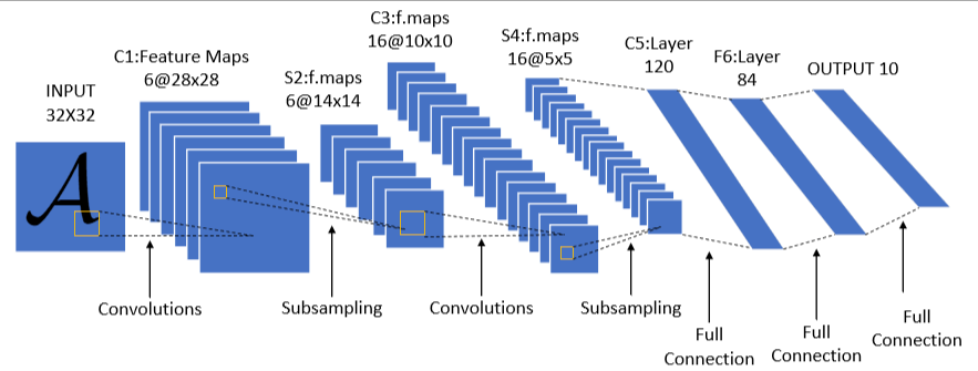
上图是LetNet-5的经典结构，它一共有七层（不包含输入层），分别是两个卷积层，两个池化层，3个全连接层（最后一个为输出层）。

层	类型	配置	输出尺寸
layer1	卷积	6 核，5×5，stride=1	6@28×28
layer2	池化	2×2，stride=2	6@14×14
layer3	卷积	16 核，5×5，stride=1	16@10×10
layer4	池化	2×2，stride=2	16@5×5
layer5	卷积	120 核，5×5，stride=1	120@1×1
layer6	全连接	120→84	84
layer7	全连接	84→10	10

注意 ：layer5 在原始论文中是卷积层，但因输出 1×1，功能等效全连接，所以常被简化为"2 卷积 +3 全连接"

2.2针对 FashionMNIST 的调整

特性	MNIST（原始）	FashionMNIST（本次）
图像尺寸	32×32（补边后）	28×28
通道数	1（灰度）	1（灰度）✓
分类数	10（数字 0-9）	10（服装类别）✓
调整	-	输入改为 28×28，去掉补边

2.3Letnet5分类部分分析

output_size = floor((input_size + 2*padding - kernel_size) / stride) + 1

层	通道数	参数	输入尺寸	计算过程	输出尺寸
Conv1	1->6	k=5,s=1,p=0	28x28	(28 - 5) // 1 + 1=24	24x24
Pool	6->6	k=2,s=2	24x24	(24 - 2) // 2 + 1=12	12x12
Conv2	6->16	k=5,s=1,p=0	12x12	(12 - 5) // 1 + 1=8	8x8
Pool2	16->16	k=2,s=2	8x8	(8 - 2) // 2 + 1=4	4x4

# 前面特征提取完后，到了全连接层，其输入是C*H*W
nn.Linear(in_features=16*4*4, out_features=120)

2.4代码实现

2.4.1目录结构

lenet_mnist/
├── data.py               # 数据加载模块
├── model.py              # LeNet-5 模型定义
├── train.py              # 训练脚本
├── eval.py               # 单张图片推理脚本
├── utils.py              # 可视化工具
├── extract_samples.py    # 提取样本图片脚本
├── README.md             # 项目说明文档
│
├── data/                 # FashionMNIST 数据集
├── samples/              # 提取的样本图片
└── outputs/              # 训练输出
    ├── lenet5_fashionmnist.pth   # 训练好的模型
    ├── training_curves.png       # 训练曲线图
    └── predictions.png            # 预测结果可视化

2.4.2 data.py

from torchvision import datasets, transforms
from torch.utils.data import DataLoader

def get_dataloaders(batch_size=64):
    """加载 FashionMNIST 数据集"""
    
    # 数据预处理
    transform = transforms.Compose([
        transforms.ToTensor(),
        transforms.Normalize((0.2860,), (0.3530,))  # FashionMNIST 均值和标准差
    ])
    
    # 下载并加载数据
    train_dataset = datasets.FashionMNIST(
        root='./data',
        train=True,
        download=True,
        transform=transform
    )
    
    test_dataset = datasets.FashionMNIST(
        root='./data',
        train=False,
        download=True,
        transform=transform
    )
    
    train_loader = DataLoader(train_dataset, batch_size=batch_size, shuffle=True, num_workers=2)
    test_loader = DataLoader(test_dataset, batch_size=batch_size, shuffle=False, num_workers=2)
    
    return train_loader, test_loader

2.4.3 model.py

import torch.nn as nn

class LeNet5(nn.Module):
    def __init__(self, num_classes=10):
        super(LeNet5, self).__init__()

        # 特征提取部分（卷积 + 池化）
        self.features = nn.Sequential(
            nn.Conv2d(in_channels=1, out_channels=6, kernel_size=5, stride=1, padding=0),
            nn.Sigmoid(),
            nn.AvgPool2d(kernel_size=2, stride=2),
            nn.Conv2d(in_channels=6, out_channels=16, kernel_size=5, stride=1, padding=0),
            nn.Sigmoid(),
            nn.AvgPool2d(kernel_size=2, stride=2)
        )
        # 分类器部分（全连接）
        self.classifier = nn.Sequential(
            nn.Linear(in_features=16*4*4, out_features=120),
            nn.Sigmoid(),
            nn.Linear(in_features=120, out_features=84),
            nn.Sigmoid(),
            nn.Linear(in_features=84, out_features=num_classes)
        )

    def forward(self, x):
        x = self.features(x)
        x = x.view(x.size(0), -1)   # 展平
        x = self.classifier(x)
        return x

2.4.4 utils.py

import matplotlib.pyplot as plt
import numpy as np
import os

def plot_training_curves(train_losses, test_losses, train_accs, test_accs, output_dir='./outputs'):
    """绘制训练曲线"""
    fig, (ax1, ax2) = plt.subplots(1, 2, figsize=(14, 5))

    # 损失曲线
    ax1.plot(train_losses, 'b-', label='Train Loss', linewidth=2)
    ax1.plot(test_losses, 'r-', label='Test Loss', linewidth=2)
    ax1.set_xlabel('Epoch')
    ax1.set_ylabel('Loss')
    ax1.set_title('Training & Test Loss')
    ax1.legend()
    ax1.grid(True, alpha=0.3)

    # 准确率曲线
    ax2.plot(train_accs, 'b-', label='Train Acc', linewidth=2)
    ax2.plot(test_accs, 'g-', label='Test Acc', linewidth=2)
    ax2.set_xlabel('Epoch')
    ax2.set_ylabel('Accuracy (%)')
    ax2.set_title('Training & Test Accuracy')
    ax2.legend()
    ax2.grid(True, alpha=0.3)

    plt.tight_layout()
    plt.savefig(os.path.join(output_dir, 'training_curves.png'), dpi=150)
    plt.show()

def visualize_predictions(model, loader, device, output_dir='./outputs', num_samples=10):
    """可视化预测结果"""
    model.eval()
    data_iter = iter(loader)
    images, labels = next(data_iter)

    images, labels = images[:num_samples].to(device), labels[:num_samples]
    outputs = model(images)
    preds = outputs.argmax(dim=1).cpu()

    # FashionMNIST 类别名称
    class_names = ['T-shirt', 'Trouser', 'Pullover', 'Dress', 'Coat',
                   'Sandal', 'Shirt', 'Sneaker', 'Bag', 'Ankle boot']

    fig, axes = plt.subplots(2, 5, figsize=(15, 6))
    axes = axes.flatten()

    for i, ax in enumerate(axes):
        # 反归一化
        img = images[i].cpu().squeeze()
        img = img * 0.3530 + 0.2860
        img = img.clamp(0, 1)

        ax.imshow(img, cmap='gray')
        true_label = class_names[labels[i]]
        pred_label = class_names[preds[i]]
        color = 'green' if preds[i] == labels[i] else 'red'
        ax.set_title(f'True: {true_label}\nPred: {pred_label}', color=color, fontsize=10)
        ax.axis('off')

    plt.tight_layout()
    plt.savefig(os.path.join(output_dir, 'predictions.png'), dpi=150)
    plt.show()

def visualize_feature_maps(model, loader, device):
    """可视化特征图"""
    model.eval()
    data_iter = iter(loader)
    images, _ = next(data_iter)
    image = images[:1].to(device)
    
    # 提取 C1、C3、C5 层特征
    feature_layers = [0, 4, 8]  # C1, C3, C5 在 features 中的索引
    layer_names = ['C1 (6@24×24)', 'C3 (16@12×12)', 'C5 (120@1×1)']
    
    fig, axes = plt.subplots(1, 3, figsize=(15, 5))
    
    for idx, (layer_idx, name) in enumerate(zip(feature_layers, layer_names)):
        with torch.no_grad():
            feature = model.get_feature_map(image, layer_idx)
        
        if idx < 2:  # C1, C3
            # 显示前几个通道
            num_channels = min(6, feature.shape[1])
            feature_grid = feature[0, :num_channels].cpu()
            
            # 创建网格
            rows = int(np.ceil(np.sqrt(num_channels)))
            fig_single, axes_single = plt.subplots(rows, rows, figsize=(8, 8))
            if rows == 1:
                axes_single = [axes_single]
            axes_single = axes_single.flatten()
            
            for ch in range(num_channels):
                f = feature_grid[ch]
                f = (f - f.min()) / (f.max() - f.min())  # 归一化到 0-1
                axes_single[ch].imshow(f, cmap='viridis')
                axes_single[ch].set_title(f'Channel {ch}')
                axes_single[ch].axis('off')
            
            for ch in range(num_channels, rows*rows):
                axes_single[ch].axis('off')
            
            plt.suptitle(f'{name} Feature Maps')
            plt.tight_layout()
            plt.savefig(f'feature_maps_layer{idx}.png', dpi=150)
            plt.show()
        else:  # C5
            print(f"{name}: 形状 {feature.shape}")
    
    plt.close('all')

2.4.5 train.py

import torch
from model import LeNet5
from data import get_dataloaders
from torch import nn
import torch.optim as optim
from utils import plot_training_curves, visualize_predictions
import os

# 输出目录
OUTPUT_DIR = './outputs'
os.makedirs(OUTPUT_DIR, exist_ok=True)

def train(model, device, train_loader, optimizer, criterion):
    model.train()
    total_loss = 0
    correct = 0
    total = 0
    
    for batch_idx, (inputs, targets) in enumerate(train_loader):
        inputs, targets = inputs.to(device), targets.to(device)

        optimizer.zero_grad()
        output = model(inputs)
        loss = criterion(output, targets)
        loss.backward()
        optimizer.step()

        total_loss += loss.item()
        pred = output.argmax(dim=1)
        correct += (pred == targets).sum().item()
        total += targets.size(0)
    
    return total_loss / len(train_loader), 100. * correct / total

def evaluate(model, device, test_loader, criterion):
    model.eval()
    total_loss, correct, total = 0, 0, 0
    
    with torch.no_grad():
        for inputs, targets in test_loader:
            inputs, targets = inputs.to(device), targets.to(device)
            output = model(inputs)
            total_loss += criterion(output, targets).item()
            pred = output.argmax(dim=1)
            correct += (pred == targets).sum().item()
            total += targets.size(0)
    
    return total_loss / len(test_loader), 100. * correct / total


def main():
    # 配置
    DEVICE = torch.device("cuda" if torch.cuda.is_available() else "cpu")
    BATCH_SIZE = 64
    EPOCHS = 10
    LR = 0.001
    
    print(f"使用设备：{DEVICE}")
    
    # 加载数据
    train_loader, test_loader = get_dataloaders(BATCH_SIZE)
    
    # 初始化模型
    model = LeNet5(num_classes=10).to(DEVICE)
    criterion = nn.CrossEntropyLoss()
    optimizer = optim.Adam(model.parameters(), lr=LR)
    scheduler = optim.lr_scheduler.StepLR(optimizer, step_size=5, gamma=0.5)
    
    # 打印模型结构
    print("\n 模型结构：")
    print(model)
    
    # 统计参数量
    total_params = sum(p.numel() for p in model.parameters())
    trainable_params = sum(p.numel() for p in model.parameters() if p.requires_grad)
    print(f"\n总参数量：{total_params:,}")
    print(f"可训练参数：{trainable_params:,}")
    
    # 训练记录
    train_losses, test_losses = [], []
    train_accs, test_accs = [], []
    
    # 训练循环
    print("\n" + "="*60)
    for epoch in range(1, EPOCHS + 1):
        train_loss, train_acc = train(model, DEVICE, train_loader, optimizer, criterion)
        test_loss, test_acc = evaluate(model, DEVICE, test_loader, criterion)
        scheduler.step()
        
        train_losses.append(train_loss)
        test_losses.append(test_loss)
        train_accs.append(train_acc)
        test_accs.append(test_acc)
        
        print(f"\nEpoch {epoch:2d}/{EPOCHS}")
        print(f"  Train Loss: {train_loss:.4f} | Train Acc: {train_acc:.2f}%")
        print(f"  Test  Loss: {test_loss:.4f} | Test  Acc: {test_acc:.2f}%")
    
    # 保存模型
    model_path = os.path.join(OUTPUT_DIR, 'lenet5_fashionmnist.pth')
    torch.save(model.state_dict(), model_path)
    print(f"\n模型已保存：{model_path}")
    
    # 可视化训练曲线
    plot_training_curves(train_losses, test_losses, train_accs, test_accs, OUTPUT_DIR)

    # 可视化预测结果
    visualize_predictions(model, test_loader, DEVICE, OUTPUT_DIR)
    
    return model

if __name__ == "__main__":
    main()

2.4.6 extract_samples.py

"""提取 FashionMNIST 图片样本"""
import os
import torch
from torchvision import datasets, transforms
from PIL import Image

# 创建输出目录
output_dir = './samples'
os.makedirs(output_dir, exist_ok=True)

# 使用不带归一化的 transform 来获取原始图片
transform = transforms.ToTensor()

# 加载测试集
test_dataset = datasets.FashionMNIST(
    root='./data',
    train=False,
    download=True,
    transform=transform
)

# FashionMNIST 类别名称
class_names = [
    'T-shirt/top', 'Trouser', 'Pullover', 'Dress', 'Coat',
    'Sandal', 'Shirt', 'Sneaker', 'Bag', 'Ankle boot'
]

# 提取每类一张图片
num_classes = 10
extracted = {i: None for i in range(num_classes)}

for idx in range(len(test_dataset)):
    img, label = test_dataset[idx]
    if extracted[label] is None:
        extracted[label] = (img, idx)
    if all(v is not None for v in extracted.values()):
        break

# 保存图片
for label, (img, idx) in extracted.items():
    # 转换为 PIL Image (img shape: [1, 28, 28])
    img_pil = transforms.ToPILImage()(img)
    filename = f'{label:02d}_{class_names[label].replace("/", "_")}.png'
    img_pil.save(os.path.join(output_dir, filename))
    print(f'Saved: {filename} (index: {idx})')

print(f'\n所有图片已保存到 {output_dir} 目录')

2.4.7 eval.py

"""单张图片推理脚本"""
import torch
import torch.nn.functional as F
from torchvision import transforms
from PIL import Image
from model import LeNet5
import os

# FashionMNIST 类别名称
CLASS_NAMES = [
    'T-shirt/top', 'Trouser', 'Pullover', 'Dress', 'Coat',
    'Sandal', 'Shirt', 'Sneaker', 'Bag', 'Ankle boot'
]

# 数据预处理（与训练时一致）
transform = transforms.Compose([
    transforms.ToTensor(),
    transforms.Normalize((0.2860,), (0.3530,))
])


def load_model(model_path='outputs/lenet5_fashionmnist.pth'):
    """加载训练好的模型"""
    device = torch.device("cuda" if torch.cuda.is_available() else "cpu")
    model = LeNet5(num_classes=10).to(device)

    if not os.path.exists(model_path):
        print(f"错误：模型文件 {model_path} 不存在")
        print("请先运行 train.py 训练模型")
        return None, device

    model.load_state_dict(torch.load(model_path, map_location=device))
    model.eval()
    print(f"模型已加载: {model_path}")
    return model, device


def predict_image(model, device, image_path):
    """对单张图片进行推理"""
    # 加载图片
    img = Image.open(image_path).convert('L')  # 转为灰度图
    img = img.resize((28, 28))  # 调整大小

    # 转为 tensor 并添加 batch 维度
    img_tensor = transform(img).unsqueeze(0).to(device)

    # 推理
    with torch.no_grad():
        output = model(img_tensor)
        probs = F.softmax(output, dim=1)
        probs = probs.squeeze()  # 移除 batch 维度

    return probs.cpu().numpy()


def print_predictions(probs, top_k=3):
    """打印各类别概率"""
    print("\n" + "=" * 50)
    print(f"Top {top_k} 类别概率:")
    print("-" * 50)

    # 按概率排序显示
    sorted_indices = sorted(range(len(probs)), key=lambda i: probs[i], reverse=True)[:top_k]

    for idx in sorted_indices:
        bar_len = int(probs[idx] * 30)
        bar = "#" * bar_len + "=" * (30 - bar_len)
        print(f"{CLASS_NAMES[idx]:12s} | {probs[idx]*100:5.2f}% | {bar}")

    print("=" * 50)


def main(image_path):
    # 加载模型
    model, device = load_model()
    if model is None:
        return

    # 检查图片路径
    if not os.path.exists(image_path):
        print(f"错误：图片文件 {image_path} 不存在")
        return

    print(f"\n推理图片: {image_path}")

    # 推理并打印结果
    probs = predict_image(model, device, image_path)
    print_predictions(probs)


if __name__ == "__main__":
    import sys

    if len(sys.argv) < 2:
        # 默认使用 samples 目录中的第一张图片
        default_path = "samples/00_T-shirt_top.png"
        if os.path.exists(default_path):
            main(default_path)
        else:
            print(f"用法: python eval.py <图片路径>")
            print(f"示例: python eval.py samples/00_T-shirt_top.png")
    else:
        main(sys.argv[1])

2.4.8 使用方法

训练模型

python train.py

训练完成后，模型和可视化结果保存在 outputs/ 目录。

单张图片推理

python eval.py samples/00_T-shirt_top.png

3.常见问题

3.1输入输出不匹配的情况

  File "/Users/whoami/miniconda3/envs/llm_develop/lib/python3.12/site-packages/torch/nn/modules/linear.py", line 125, in forward
    return F.linear(input, self.weight, self.bias)
           ^^^^^^^^^^^^^^^^^^^^^^^^^^^^^^^^^^^^^^^
RuntimeError: mat1 and mat2 shapes cannot be multiplied (64x256 and 400x120)

答：前面特征提取完后，到了全连接层，其输入是CHW，输入要与输出匹配

nn.Linear(in_features=16*4*4, out_features=120)

3.2模型改进

原始论文中激活函数使用sigmoid，但是现代letnet5一般会用relu。