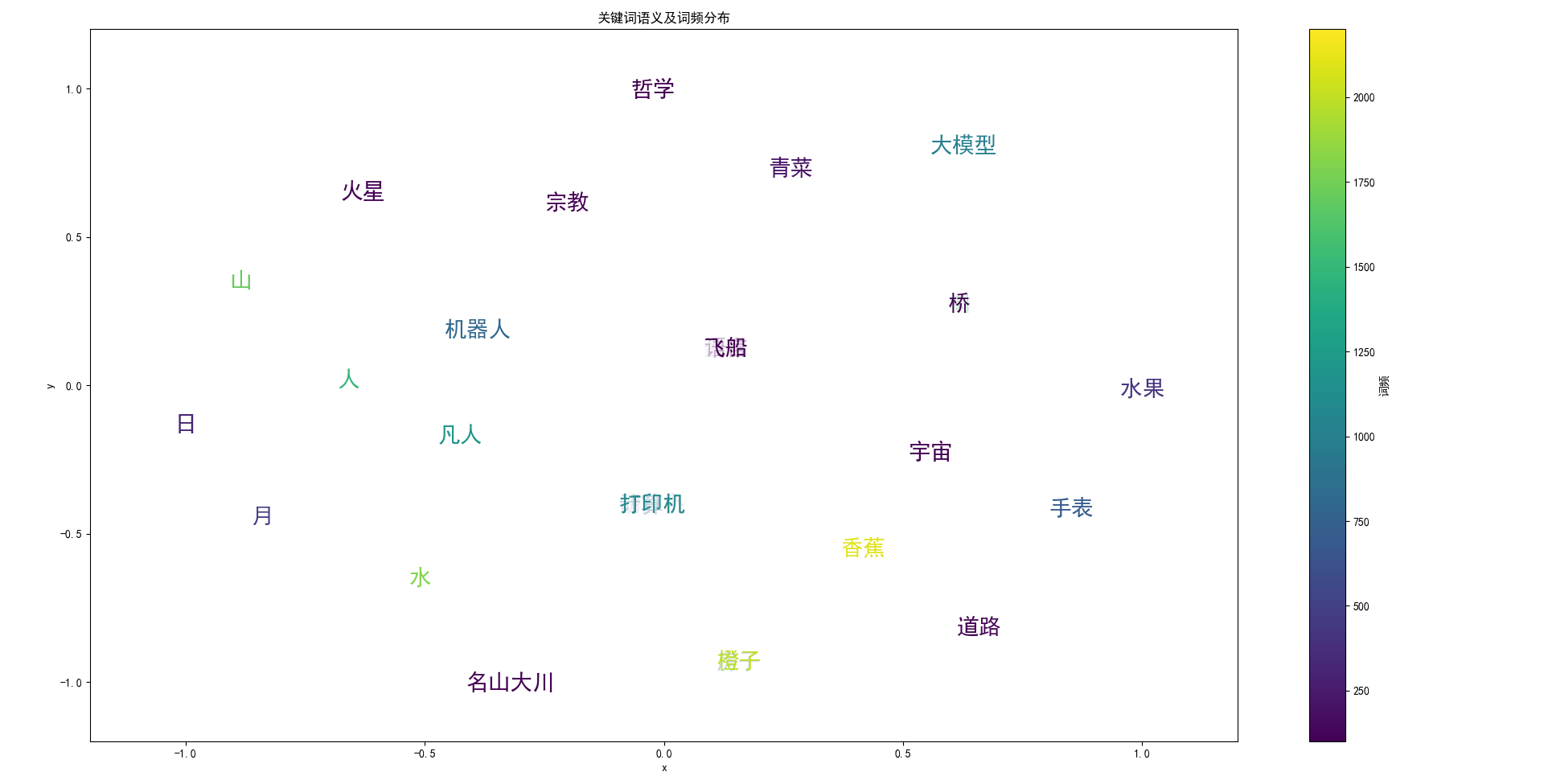
通过二维平面内的距离体现词与词的相关性,
通过词汇文本颜色的色值体现词汇的词频,
也可以通过词汇文本的字体大小来体现词频信息,
或者另一个维度的数值(时间远近)。
python
# 数据可视化
# 输入数据位词频列表
# 输出数据可视化图表
# 先将词频列表中的词汇通过chromadb存储到向量数据库中
# 然后从chromadb中提取出各个词汇的向量
# 将词频列表中各个词汇的向量降维到2维
# 然后将降维后的向量可视化到平面图中
# 将每个词汇的向量可视化到平面图中
# 词汇的频频数值通过可视化平面图中字符的颜色深浅来体现

from modelscope import snapshot_download

from sentence_transformers import SentenceTransformer
import numpy as np

# 引入向量数据库
import chromadb
# 引入降维算法
from sklearn.manifold import TSNE
# 引入可视化库
import matplotlib.pyplot as plt
from matplotlib.colors import Normalize

#----------------------------------------------
# 设置数据可视化中文字体,确保汉字能正确显示
plt.rcParams['font.sans-serif'] = ['SimHei', 'Microsoft YaHei', 'Arial Unicode MS']
plt.rcParams['axes.unicode_minus'] = False  # 解决负号显示问题
#----------------------------------------------
# 将词嵌入预训练模型下载到指定路径,供chromadb使用
model_dir = snapshot_download(
    model_id='sentence-transformers/all-MiniLM-L6-v2',
    cache_dir=r"D:\ai_models\all-MiniLM-L6-v2"
)
#----------------------------------------------
# 加载本地模型
try:
    # 尝试加载用户指定路径的模型
    model_path = r"D:\ai_models\all-MiniLM-L6-v2\sentence-transformers\all-MiniLM-L6-v2"
    model = SentenceTransformer(model_path)
    print(f"成功加载本地模型: {model_path}")
except Exception as e:
    print(f"加载本地模型失败: {e}")
    print("尝试从HuggingFace加载模型...")
    # 如果本地模型加载失败,尝试从HuggingFace加载
    model = SentenceTransformer('sentence-transformers/all-MiniLM-L6-v2')
#----------------------------------------------
# 使用以上模型给chromadb构建词嵌入程序
# 创建符合ChromaDB EmbeddingFunction接口的类
class CustomEmbeddingFunction:
    def __init__(self, model):
        self.model = model

    def __call__(self, input):
        return self.model.encode(input).tolist()
#----------------------------------------------
# 使用自定义嵌入函数
embedding_function = CustomEmbeddingFunction(model)

# 直接使用以上modelscope下载的模型将词汇向量化
def vectorize_word(word):
    """将单个词汇向量化"""
    embedding = model.encode(word)
    print(f"词汇 '{word}' 的向量: {embedding}")
    return embedding

#----------------------------------------------

# 本地创建持久化的chromadb数据库
chrome_client = chromadb.PersistentClient(path="./word_freq_chromadb")
#----------------------------------------------

def save_word_freq_to_chromadb(word_freq):

    # 删除已存在的collection
    try:
        chrome_client.delete_collection("word_freq")
    except:
        pass

    # 创建collection,指定embedding_function
    collection = chrome_client.create_collection("word_freq", embedding_function=embedding_function)

    # 向chromadb数据库中添加词汇向量
    words=[]
    meta_datas=[]
    ids=[]
    embeddings=[]

    for word_freq_item in word_freq:
        word=word_freq_item[0]
        freq=word_freq_item[1]
        # 避免重复添加
        if word in ids:
            continue
        words.append(word)
        meta_datas.append({"freq": freq})
        ids.append(word)
        embeddings.append(embedding_function(word))
        print(word,freq)

    # 向collection中添加词汇向量
    collection.add(
        documents=words,
        metadatas=meta_datas,
        ids=ids,
        embeddings=embeddings
    )
#----------------------------------------------
def visualize_word_freq():

    # 从chromadb中提取出各个词汇的向量
    collection = chrome_client.get_collection("word_freq")
    # 直接将collection中所有词极其对应向量列出
    results = collection.get(include=["documents", "embeddings", "metadatas"])
    # print(results)
    # 从results中提取出词汇、向量、频率
    words=results["documents"]
    embeddings=results["embeddings"]
    metadatas=results["metadatas"]
    freqs=[meta["freq"] for meta in metadatas]
     # 对向量进行降维
    sample_count=len(words)
    print(f"样本数量: {sample_count}")
    perplexity=min(30,sample_count-1)
    tsne = TSNE(n_components=2, random_state=42, perplexity=perplexity)
    embeddings_2d = tsne.fit_transform(embeddings)
    # 可视化,对应的二维坐标点上还要绘制对应的词汇

    # 整理数据,结构:(词汇、二维坐标点、频率)
    word_embeddings_2d=list(zip(words, embeddings_2d, freqs))
    for w in word_embeddings_2d:
        print(w)

    # 可视化,将words按照embeddings_2d中的坐标点可视化到平面图中,word的颜色值对应freq
    plt.figure(figsize=(12, 10))
    # 获取当前Axes
    ax = plt.gca()
    # 标准化坐标值到[-1, 1]范围,便于可视化
    from sklearn.preprocessing import MinMaxScaler
    scaler = MinMaxScaler(feature_range=(-1, 1))
    embeddings_2d_normalized = scaler.fit_transform(embeddings_2d)
    # 创建颜色映射
    cmap = plt.cm.viridis
    norm = Normalize(vmin=min(freqs), vmax=max(freqs))

    # 在每个点的位置绘制词汇,词汇颜色对应词频
    for i, (word, freq) in enumerate(zip(words, freqs)):
        x, y = embeddings_2d_normalized[i]
        # 设置词汇颜色,使用词频映射到颜色
        color = cmap(norm(freq))
        print(f"绘制词汇: {word}, 坐标: ({x}, {y}), 词频: {freq}, 颜色: {color}")
        # 先绘制一个小散点,确保位置正确
        # ax.scatter(x, y, color=color, alpha=0.5, s=100)
        # 绘制词汇,使用更大的字体
        # 绘制词汇,使用更大的字体
        ax.text(x, y, word, fontsize=20, ha='center', va='center',
               color=color, fontweight='bold',
               bbox=dict(facecolor='white', alpha=0.7, edgecolor='none', boxstyle='round,pad=0.3'))

    # 添加颜色条
    sm = plt.cm.ScalarMappable(cmap=cmap, norm=norm)
    sm.set_array([])
    plt.colorbar(sm, ax=ax, label='词频')

    # 完成绘制
    plt.title("关键词语义及词频分布")
    plt.xlabel("x")
    plt.ylabel("y")
    # plt.grid(True, linestyle='--', alpha=1)
    # 设置坐标轴范围
    plt.xlim(-1.2, 1.2)
    plt.ylim(-1.2, 1.2)

    plt.tight_layout()
    plt.show()

#----------------------------------------------
if __name__ == "__main__":
    word_freq=[("胡萝卜",100),("青菜",200),("日",300),("水果",400),("月",500),("时钟",600),("手表",700),("机器人",800),("汽车",900), ("房子",1000),("圣贤",1100), ("凡人",1200),("猫",1300),("狗",1400),("人",1500),("树",1600),("山",1700),("水",1800),("苹果",1900),("橙子",2000),("香蕉",2100),("汽油",2200),("书籍",1000),("计算机",800),("咖啡",200),("蛋糕",100),("桥",100),("道路",100),("打印机",1100),("大模型",1000),("哲学",100),("宗教",100),("语言",100),("名山大川",100),("宇宙",100),("飞船",100),("火星",100)]

    # vectorize_word("天")
    save_word_freq_to_chromadb(word_freq)
    visualize_word_freq()
    pass