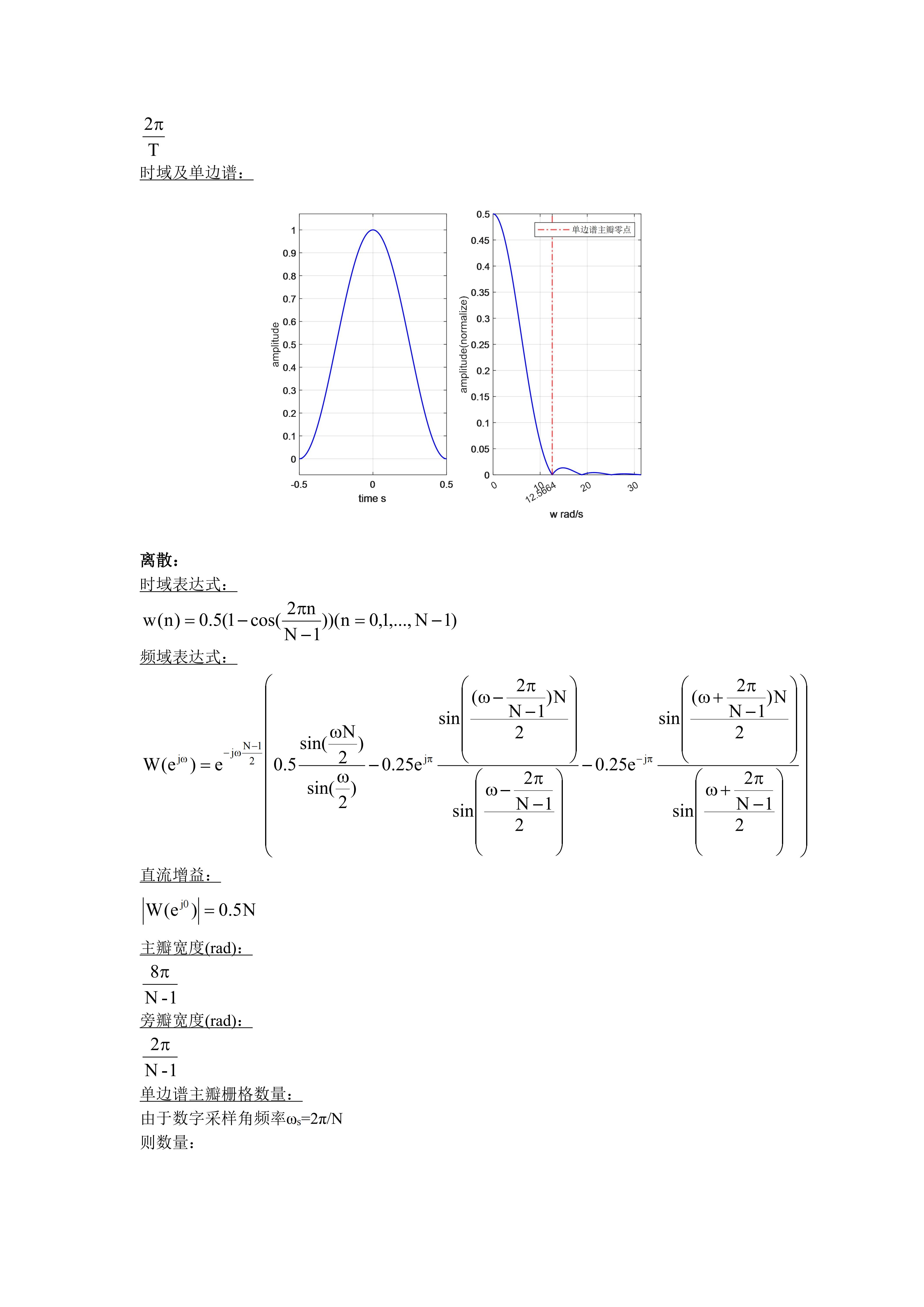
狭义的信号S(t)是以时间为自变量的一维函数,则定义域是无穷,只要时间存在信号便存在,而我们对信号的捕获天然是局部的,这种局部视为"窗函数"与源信号在时间的乘积,而窗函数作为非平稳性质的确定性能量信号,有诸多形式存在:矩形、三角形、汉明、汉宁...只要是个类似的能量函数都叫做窗函数,但最具代表性的窗函数往往具备在信号分析中具有特别优势,下面分别介绍两种:
关于上面的GIF图如下:
涉及MATLAB程序如下:
Matlab
clc;clear;close all
fs = 10;    % 采样率
T = 1/fs;   % 采样周期
wT = 1;     % 窗口连续时间
wN = wT*fs; % 窗口离散点数
winN = 30;  % 动图窗长
f_range = linspace(-fs/2,fs/2,1e3);
A_arr = zeros(1,1e3);
f1_ridx = 1e3/2+1e2+1;
f2_ridx = 1e3/2+1.5e2+1;
f1_lidx = 1e3/2-1e2;
f2_lidx = 1e3/2-1.5e2;
f1 = fs/1e3*1e2;
f2 = fs/1e3*1.5e2;
disp(['频率1:',num2str(f1),'Hz']);
disp(['频率2:',num2str(f2),'Hz'])
A_arr([f1_lidx,f1_ridx]) = 1;
A_arr([f2_lidx,f2_ridx]) = 1.5;
figure
plot(f_range,A_arr,'LineWidth',1,'Color','blue');
xlim('tight')
ylim('padded')
xlabel('频率 Hz')
ylabel('幅度')
grid
box
%% 矩形窗
% 连续
t = linspace(-wT/2,wT/2,1e4);
At = ones(1,length(t));
w = linspace(0,10*pi,1e4);
Aw = wT*abs(sin(0.5*wT*w(2:end))./(0.5*wT*w(2:end)));
Aw = [wT,Aw];
figure
subplot(121)
plot(t,At,'LineWidth',1,'Color','blue');
xlim('tight')
ylim('padded')
xlabel('time s')
ylabel('amplitude')
grid on
subplot(122)
plot(w,Aw/wT,'LineWidth',1,'Color','blue','HandleVisibility','off');
hold on
xline(2*pi/wT,'LineWidth',1,'LineStyle','-.','Color','red','DisplayName','单边谱主瓣零点');
xlim('tight')
xt = xticks;
xticks(sort([2*pi/wT, xt]));
xlabel('w rad/s')
ylabel('amplitude(normalize)')
grid on
legend
disp('矩形窗(连续):')
disp(['主瓣宽度:',num2str(4*pi/wT),'rad/s']);

% 离散
An = ones(1,wN);
w = linspace(0,pi,1e4);
Aw = abs(sin(0.5*w*wN)./sin(0.5*w));
Aw(1) = wN;
figure
subplot(121)
stem(0:wN - 1,An,'Color','blue','Marker','o','MarkerSize',5,'MarkerEdgeColor','red','MarkerFaceColor','white');
xlim('tight')
ylim('padded')
xlabel('samples')
ylabel('amplitude')
grid on
subplot(122)
plot(w,Aw/wN,'Color','blue','LineWidth',1,'HandleVisibility','off');
xline(2*pi/wN,'LineWidth',1,'LineStyle','-.','Color','red','DisplayName','单边主瓣零点');


w = (0:fs/wN:fs/2)*2*pi;
Aw = abs(sin(wN*T*w/2)./sin(T*w/2));
Aw(1) = wN;
hold on
stem(w/fs,Aw/wN,'LineWidth',1,'Color','blue','Marker','o','MarkerSize',5,'HandleVisibility','off', ...
    'MarkerEdgeColor','red','MarkerFaceColor','white');
xt = xticks;
xticks(sort([2*pi/wN, xt]));
xlim('tight')
xlabel('w rad')
ylabel('amplitude(normalize)');
grid on
legend
% 卷积
w = linspace(-pi,pi,1e3);
A_conved = sin(0.5*w*winN)./sin(0.5*w);

A_conved = A_conved / max(A_conved);
rect_conv = abs(conv(A_conved,A_arr));
conv_res = zeros(1,length(rect_conv));
conv_pro = [A_conved,zeros(1,length(A_arr) - 1)];

figure
subplot(211)
fig1 = plot(linspace(-fs,fs,length(conv_res)),conv_res,'LineWidth',1,'Color','blue');
xlim('tight')
ylim([-0.25,max(rect_conv)*1.5])
grid on
ylabel('Amplitude')
xlabel('Frequence Hz')
subplot(212)

plot(1:length(conv_pro),[zeros(1,length(A_conved) - 1),A_arr],'LineWidth',1,'Color','red');hold on
fig2 = plot(1:length(conv_pro),conv_pro,'LineWidth',1,'Color','blue');
xlim('tight');
ylim([-0.25,2]);
grid on
ylabel('Amplitude')
xlabel('Delay')
F1 = getframe(gcf);
I1 = frame2im(F1);
[I1,map1]=rgb2ind(I1,256);
imwrite(I1,map1,'gif1.gif','gif','Loopcount',inf,'DelayTime',0.005);
speed = 10;
for i = 2:length(rect_conv) / speed
    fig1.YData(1:i * speed) = rect_conv(1:i * speed);
    fig2.YData = [zeros(1,speed), fig2.YData(1:end - speed)];
    pause(0.1);
    F1 = getframe(gcf);
    I1 = frame2im(F1);
    [I1,map1]=rgb2ind(I1,256);
    imwrite(I1,map1,'gif1.gif','gif','WriteMode','append','DelayTime',0.005);
end
t = (0:winN - 1) / fs;
s = 1*cos(2*pi*f1*t) + 1.5*cos(2*pi*f2*t);
fft_res = fft(s);
fft_res = fftshift(abs(fft_res) / winN * 2);
figure
stem(linspace(-fs/2,fs/2,length(fft_res)),fft_res,'LineWidth',1,'Color','blue','Marker','.','MarkerSize',5);
xlim('tight')
grid on
box on
xlabel('Frequence Hz')
ylabel('Amplitude')
figure
conv_res = rect_conv(length(A_conved) / 2:length(rect_conv) - length(A_conved) / 2);
plot(f_range,conv_res,'LineWidth',1,'Color','blue');
hold on
plot(f_range,A_arr,'LineWidth',1,'Color','red');
grid on
box on
xlim('tight');
xlabel('Frequence Hz')
ylabel('Amplitude')
%% 汉宁窗
% 连续
t = linspace(-wT/2,wT/2,1e4);
At = 0.5*(1+cos(2*pi*t/wT));
w = linspace(0,10*pi,1e4);
Aw = wT*abs(0.5*sin(w(2:end)*wT/2)./(w(2:end)*wT/2) + ...
    0.25*sin(w(2:end)*wT/2 - pi)./(w(2:end)*wT/2 - pi) + ...
    0.25*sin(w(2:end)*wT/2 + pi)./(w(2:end)*wT/2 + pi));
Aw = [wT / 2,Aw];
figure
subplot(121)
plot(t,At,'LineWidth',1,'Color','blue');
xlim('tight')
ylim('padded')
xlabel('time s')
ylabel('amplitude')
grid on
subplot(122)
plot(w,Aw/wT,'LineWidth',1,'Color','blue','HandleVisibility','off');
hold on
xline(4*pi/wT,'LineWidth',1,'LineStyle','-.','Color','red','DisplayName','单边谱主瓣零点');
xlim('tight')
xt = xticks;
xticks(sort([4*pi/wT, xt]));
xlabel('w rad/s')
ylabel('amplitude(normalize)')
grid on
legend
disp('汉宁窗(连续):')
disp(['主瓣宽度:',num2str(8*pi/wT),'rad/s']);

% 离散
n = 0:wN - 1;
An = 0.5*(1-cos(2*pi*n/(wN - 1)));
w = linspace(0,pi,1e4);
X = 2*pi/(wN - 1);

D0 = sin(wN*w/2) ./ sin(w/2);
D0(isnan(D0)) = wN;

Dp = sin(wN*(w-X)/2) ./ sin((w-X)/2);
Dp(isnan(Dp)) = wN;

Dm = sin(wN*(w+X)/2) ./ sin((w+X)/2);
Dm(isnan(Dm)) = wN;

Aw = abs(0.5*D0 + 0.25*Dp + 0.25*Dm);

figure
subplot(121)
stem(0:wN - 1,An,'Color','blue','Marker','o','MarkerSize',5,'MarkerEdgeColor','red','MarkerFaceColor','white');
xlim('tight')
ylim('padded')
xlabel('samples')
ylabel('amplitude')
grid on
subplot(122)
plot(w,Aw/wN,'LineWidth',1,'Color','blue','HandleVisibility','off'); grid on
xline(4*pi/(wN - 1)*wN/wN,'LineStyle','-.','Color','red','DisplayName','单边谱主瓣零点');
w = (0:fs/wN:fs/2)*2*pi;
X = 2*pi/(wN - 1);

D0 = sin(wN*w*T/2) ./ sin(w*T/2);
D0(isnan(D0)) = wN;

Dp = sin(wN*(w*T-X)/2) ./ sin((w*T-X)/2);
Dp(isnan(Dp)) = wN;

Dm = sin(wN*(w*T+X)/2) ./ sin((w*T+X)/2);
Dm(isnan(Dm)) = wN;

Aw = abs(0.5*D0 + 0.25*Dp + 0.25*Dm);
hold on
stem(w/fs,Aw/wN,'LineWidth',1,'Color','blue','Marker','o','MarkerSize',5,'HandleVisibility','off', ...
    'MarkerEdgeColor','red','MarkerFaceColor','white');
xlim('tight')
xt = xticks;
xticks(sort([4*pi/(wN - 1), xt]));
xlabel('w rad')
ylabel('amplitude(normalize)')
grid on
legend

% 卷积
w = linspace(-pi,pi,1e3);
X = 2*pi/(winN - 1);

D0 = sin(winN*w/2) ./ sin(w/2);
D0(isnan(D0)) = winN;

Dp = sin(winN*(w-X)/2) ./ sin((w-X)/2);
Dp(isnan(Dp)) = winN;

Dm = sin(winN*(w+X)/2) ./ sin((w+X)/2);
Dm(isnan(Dm)) = winN;

A_conved = 0.5*D0 + 0.25*Dp + 0.25*Dm;
A_conved = A_conved / max(A_conved);
hann_conv = abs(conv(A_conved,A_arr));
conv_res = zeros(1,length(hann_conv));
conv_pro = [A_conved,zeros(1,length(A_arr) - 1)];

figure
subplot(211)
fig1 = plot(linspace(-fs,fs,length(conv_res)),conv_res,'LineWidth',1,'Color','blue');
xlim('tight')
ylim([-0.25,max(hann_conv)*1.5])
grid on
ylabel('Amplitude')
xlabel('Frequence Hz')
subplot(212)

plot(1:length(conv_pro),[zeros(1,length(A_conved) - 1),A_arr],'LineWidth',1,'Color','red');hold on
fig2 = plot(1:length(conv_pro),conv_pro,'LineWidth',1,'Color','blue');
xlim('tight');
ylim([-0.25,2]);
grid on
ylabel('Amplitude')
xlabel('Delay')
F2 = getframe(gcf);
I2 = frame2im(F2);
[I2,map2]=rgb2ind(I2,256);
imwrite(I2,map2,'gif2.gif','gif','Loopcount',inf,'DelayTime',0.005);
speed = 10;
for i = 2:length(hann_conv) / speed
    fig1.YData(1:i * speed) = hann_conv(1:i * speed);
    fig2.YData = [zeros(1,speed), fig2.YData(1:end - speed)];
    pause(0.1);
    F2 = getframe(gcf);
    I2 = frame2im(F2);
    [I2,map2]=rgb2ind(I2,256);
    imwrite(I2,map2,'gif2.gif','gif','WriteMode','append','DelayTime',0.005);
end
t = (0:winN - 1) / fs;
n = 0:winN - 1;
win = 0.5*(1-cos(2*pi*n/(winN - 1)));
s = 1*cos(2*pi*f1*t) + 1.5*cos(2*pi*f2*t);
fft_res = fft(s .* win);
fft_res = fftshift(abs(fft_res) / winN * 4);
figure
stem(linspace(-fs/2,fs/2,length(fft_res)),fft_res,'LineWidth',1,'Color','blue','Marker','.','MarkerSize',5);
xlim('tight')
grid on
box on
xlabel('Frequence Hz')
ylabel('Amplitude')
figure
conv_res = hann_conv(length(A_conved) / 2:length(hann_conv) - length(A_conved) / 2);
plot(f_range,conv_res,'LineWidth',1,'Color','blue');
hold on
plot(f_range,A_arr,'LineWidth',1,'Color','red');
grid on
box on
xlim('tight');
xlabel('Frequence Hz')
ylabel('Amplitude')