MATLAB绘图风格记录NP类型

以下Matlab代码展示了NP类型的绘图风格，方便后续论文绘图参考，代码和演示图片如下
Matlab 复制代码
%% ============================================================
%  Nature Photonics 风格配色选型展示板 (MATLAB)
%  完整自包含版本 - 直接运行即可
%  ============================================================
close all; clear; clc;

%% ========== 配色定义 ==========
% Nature Photonics 高频配色
np.blue    = [0,   119, 187] / 255;
np.cyan    = [51,  187, 238] / 255;
np.red     = [238, 51,  119] / 255;
np.orange  = [238, 119, 51]  / 255;
np.teal    = [0,   153, 136] / 255;
np.yellow  = [236, 174, 23]  / 255;
np.indigo  = [51,  34,  136] / 255;
np.purple  = [170, 51,  119] / 255;

% Paul Tol Bright (色盲友好)
tol.blue   = [68,  119, 170] / 255;
tol.cyan   = [102, 204, 238] / 255;
tol.green  = [34,  136, 51]  / 255;
tol.yellow = [204, 187, 68]  / 255;
tol.red    = [238, 102, 119] / 255;
tol.purple = [170, 51,  119] / 255;
tol.grey   = [187, 187, 187] / 255;

% 5色调色板（快捷引用）
palette5 = [np.blue; np.red; np.orange; np.teal; np.indigo];

%% ========== 全局样式 ==========
set(0, 'DefaultAxesFontName',   'Arial');
set(0, 'DefaultAxesFontSize',   8);
set(0, 'DefaultAxesLineWidth',  0.8);
set(0, 'DefaultAxesTickDir',    'in');
set(0, 'DefaultAxesBox',        'off');
set(0, 'DefaultLineLineWidth',  1.0);
set(0, 'DefaultFigureColor',    'w');

%% ========== 生成公共数据 ==========
t = linspace(0, 20, 4000);
f = linspace(0, 50, 1000);

% 光脉冲
pulse1 = exp(-(t-5).^2 / 0.8) .* cos(2*pi*3*t);
pulse2 = exp(-(t-8).^2 / 1.5) .* cos(2*pi*3*t - 0.5) * 0.75;
pulse3 = exp(-(t-12).^2 / 0.5) .* cos(2*pi*4.5*t) * 0.6;

% 频谱
spec1 = exp(-(f-15).^2 / 3);
spec2 = exp(-(f-18).^2 / 5) * 0.8;
spec3 = exp(-(f-22).^2 / 2) * 0.5;

% 色散曲线
k = linspace(0, 10, 300);
omega1 = 2.0 * sqrt(k + 0.1);
omega2 = 1.8 * sqrt(k + 0.5) + 0.3;

%% ================================================================
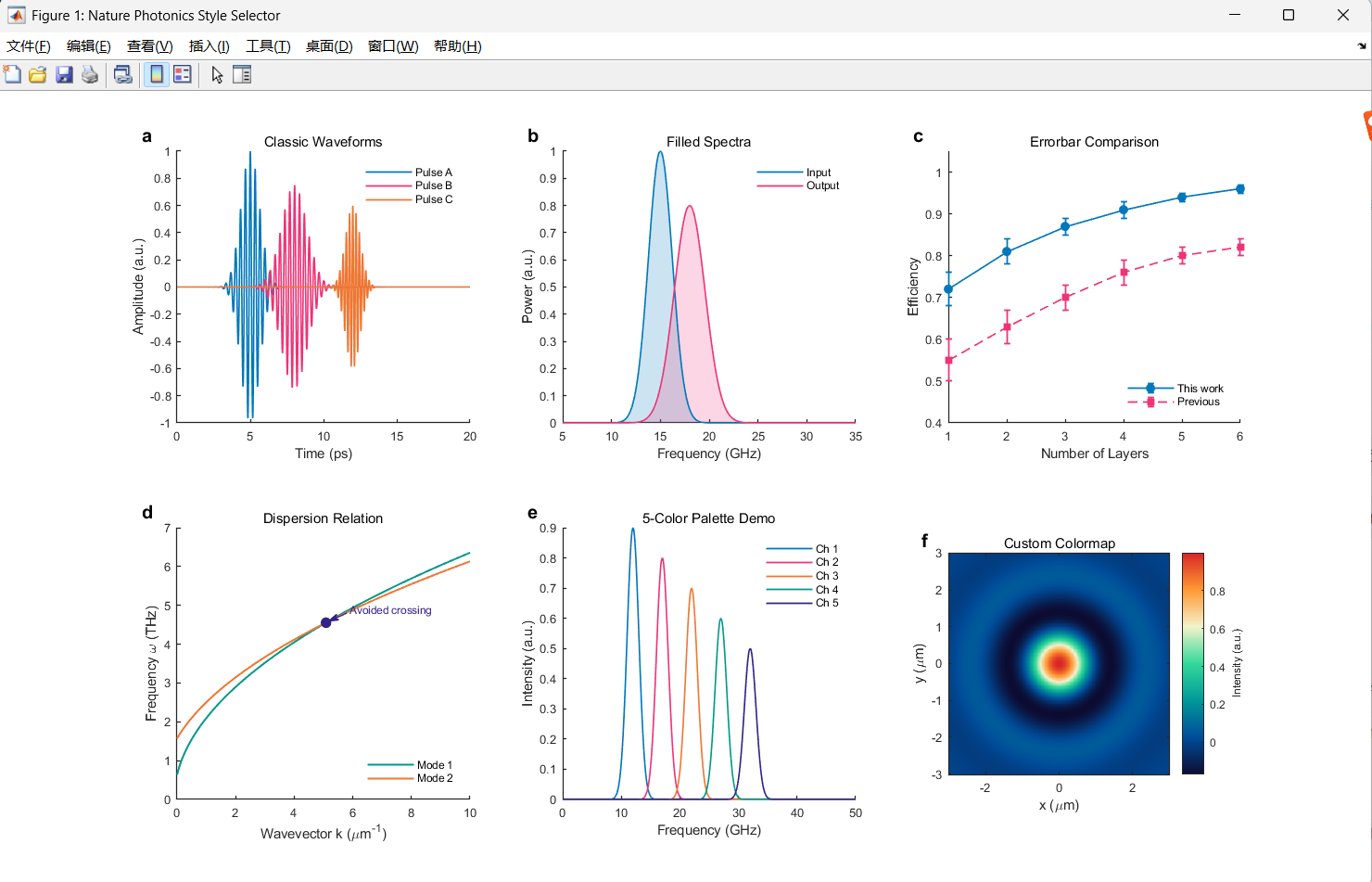
%  主图：2x3 选型展示板
%  ================================================================
fig = figure('Position', [50, 50, 1400, 850], ...
             'Name', 'Nature Photonics Style Selector');

% ==================== (a) 经典信号波形 ====================
ax_a = subplot(2,3,1);
hold on;
plot(t, pulse1, 'Color', np.blue,   'LineWidth', 1.0);
plot(t, pulse2, 'Color', np.red,    'LineWidth', 1.0);
plot(t, pulse3, 'Color', np.orange, 'LineWidth', 1.0);
hold off;
xlabel('Time (ps)');
ylabel('Amplitude (a.u.)');
xlim([0 20]);
legend({'Pulse A','Pulse B','Pulse C'}, ...
       'Location','northeast','FontSize',7,'Box','off');
% 面板标签
text(-0.12, 1.06, 'a', 'Units','normalized', ...
     'FontSize',12, 'FontWeight','bold', 'Parent',ax_a);
title('Classic Waveforms', 'FontSize',9, 'FontWeight','normal');

% ==================== (b) 填充频谱对比 ====================
ax_b = subplot(2,3,2);
hold on;
fill([f, fliplr(f)], [spec1, zeros(size(spec1))], np.blue, ...
     'FaceAlpha',0.2, 'EdgeColor','none', 'HandleVisibility','off');
fill([f, fliplr(f)], [spec2, zeros(size(spec2))], np.red, ...
     'FaceAlpha',0.2, 'EdgeColor','none', 'HandleVisibility','off');
plot(f, spec1, 'Color', np.blue, 'LineWidth', 1.0);
plot(f, spec2, 'Color', np.red,  'LineWidth', 1.0);
hold off;
xlabel('Frequency (GHz)');
ylabel('Power (a.u.)');
xlim([5 35]);
legend({'Input','Output'}, 'Location','northeast','FontSize',7,'Box','off');
text(-0.12, 1.06, 'b', 'Units','normalized', ...
     'FontSize',12, 'FontWeight','bold', 'Parent',ax_b);
title('Filled Spectra', 'FontSize',9, 'FontWeight','normal');

% ==================== (c) 散点+误差棒 ====================
ax_c = subplot(2,3,3);
x_data = 1:6;
y1 = [0.72, 0.81, 0.87, 0.91, 0.94, 0.96];
y2 = [0.55, 0.63, 0.70, 0.76, 0.80, 0.82];
e1 = [0.04, 0.03, 0.02, 0.02, 0.01, 0.01];
e2 = [0.05, 0.04, 0.03, 0.03, 0.02, 0.02];
hold on;
errorbar(x_data, y1, e1, 'o-', 'Color', np.blue, ...
         'MarkerFaceColor', np.blue, 'MarkerSize', 5, ...
         'LineWidth', 1.0, 'CapSize', 4);
errorbar(x_data, y2, e2, 's--', 'Color', np.red, ...
         'MarkerFaceColor', np.red, 'MarkerSize', 5, ...
         'LineWidth', 1.0, 'CapSize', 4);
hold off;
xlabel('Number of Layers');
ylabel('Efficiency');
ylim([0.4, 1.05]);
legend({'This work','Previous'}, 'Location','southeast','FontSize',7,'Box','off');
text(-0.12, 1.06, 'c', 'Units','normalized', ...
     'FontSize',12, 'FontWeight','bold', 'Parent',ax_c);
title('Errorbar Comparison', 'FontSize',9, 'FontWeight','normal');

% ==================== (d) 色散曲线+交叉标注 ====================
ax_d = subplot(2,3,4);
hold on;
plot(k, omega1, 'Color', np.teal,   'LineWidth', 1.2);
plot(k, omega2, 'Color', np.orange, 'LineWidth', 1.2);
% 找交叉点
[~, idx] = min(abs(omega1 - omega2));
plot(k(idx), omega1(idx), 'o', 'Color', np.indigo, ...
     'MarkerFaceColor', np.indigo, 'MarkerSize', 6);
% 标注箭头
text(k(idx)+0.8, omega1(idx)+0.35, 'Avoided crossing', ...
     'FontSize', 7, 'Color', np.indigo);
annotation('arrow', 'Color', np.indigo, 'LineWidth', 0.8, ...
           'HeadLength', 6, 'HeadWidth', 5, ...
           'Position', get_arrow_pos(ax_d, fig, k(idx)+0.7, omega1(idx)+0.25, k(idx)+0.1, omega1(idx)+0.05));
hold off;
xlabel('Wavevector k (\mum^{-1})');
ylabel('Frequency \omega (THz)');
legend({'Mode 1','Mode 2'}, 'Location','southeast','FontSize',7,'Box','off');
text(-0.12, 1.06, 'd', 'Units','normalized', ...
     'FontSize',12, 'FontWeight','bold', 'Parent',ax_d);
title('Dispersion Relation', 'FontSize',9, 'FontWeight','normal');

% ==================== (e) 多线对比（5色调色板） ====================
ax_e = subplot(2,3,5);
hold on;
labels_e = {};
for ii = 1:5
    shift = (ii-1)*5;
    sig = exp(-(f - 12 - shift).^2 / 2) * (1 - 0.1*ii);
    plot(f, sig, 'Color', palette5(ii,:), 'LineWidth', 1.0);
    labels_e{ii} = sprintf('Ch %d', ii);
end
hold off;
xlabel('Frequency (GHz)');
ylabel('Intensity (a.u.)');
xlim([0 50]);
legend(labels_e, 'Location','northeast','FontSize',7,'Box','off');
text(-0.12, 1.06, 'e', 'Units','normalized', ...
     'FontSize',12, 'FontWeight','bold', 'Parent',ax_e);
title('5-Color Palette Demo', 'FontSize',9, 'FontWeight','normal');

% ==================== (f) 2D colormap 热力图 ====================
ax_f = subplot(2,3,6);
[X, Y] = meshgrid(linspace(-3,3,300), linspace(-3,3,300));
Z = sinc(sqrt(X.^2 + Y.^2)) .* exp(-(X.^2 + Y.^2)/8);
imagesc(linspace(-3,3,300), linspace(-3,3,300), Z);
axis xy equal tight;
colormap(ax_f, nat_photonics_cmap());
cb = colorbar;
cb.Label.String = 'Intensity (a.u.)';
cb.Label.FontSize = 7;
xlabel('x (\mum)');
ylabel('y (\mum)');
text(-0.12, 1.06, 'f', 'Units','normalized', ...
     'FontSize',12, 'FontWeight','bold', 'Parent',ax_f);
title('Custom Colormap', 'FontSize',9, 'FontWeight','normal');

%% ========== 调整整体布局并保存 ==========
set(fig, 'PaperPositionMode', 'auto');
% 保存
print(fig, 'NP_style_selector', '-dpng', '-r300');
% print(fig, 'NP_style_selector', '-dpdf');  % 矢量版
fprintf('✅ 图片已保存: NP_style_selector.png\n');

%% ================================================================
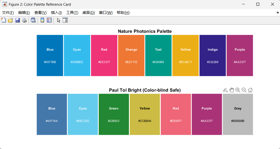
%  图2：调色板色卡展示
%  ================================================================
fig2 = figure('Position', [100, 100, 900, 400], ...
              'Name', 'Color Palette Reference Card');

% --- Nature Photonics 主色 ---
subplot(2,1,1);
np_colors = [np.blue; np.cyan; np.red; np.orange; np.teal; np.yellow; np.indigo; np.purple];
np_names  = {'Blue','Cyan','Red','Orange','Teal','Yellow','Indigo','Purple'};
np_hex    = {'#0077BB','#33BBEE','#EE3377','#EE7733','#009988','#ECAE17','#332288','#AA3377'};
for ii = 1:8
    rectangle('Position', [ii-1, 0, 1, 1], ...
              'FaceColor', np_colors(ii,:), 'EdgeColor', 'w', 'LineWidth', 2);
    text(ii-0.5, 0.65, np_names{ii}, 'HorizontalAlignment','center', ...
         'FontSize', 8, 'FontWeight','bold', 'Color','w');
    text(ii-0.5, 0.35, np_hex{ii}, 'HorizontalAlignment','center', ...
         'FontSize', 7, 'Color','w');
end
xlim([0 8]); ylim([0 1]);
axis off;
title('Nature Photonics Palette', 'FontSize', 11, 'FontWeight', 'bold');

% --- Paul Tol Bright ---
subplot(2,1,2);
tol_colors = [tol.blue; tol.cyan; tol.green; tol.yellow; tol.red; tol.purple; tol.grey];
tol_names  = {'Blue','Cyan','Green','Yellow','Red','Purple','Grey'};
tol_hex    = {'#4477AA','#66CCEE','#228833','#CCBB44','#EE6677','#AA3377','#BBBBBB'};
for ii = 1:7
    rectangle('Position', [ii-0.5-0.5, 0, 1, 1], ...
              'FaceColor', tol_colors(ii,:), 'EdgeColor', 'w', 'LineWidth', 2);
    text_color = 'w';
    if ii == 4 || ii == 7, text_color = 'k'; end  % 亮色背景用黑字
    text(ii-0.5, 0.65, tol_names{ii}, 'HorizontalAlignment','center', ...
         'FontSize', 8, 'FontWeight','bold', 'Color', text_color);
    text(ii-0.5, 0.35, tol_hex{ii}, 'HorizontalAlignment','center', ...
         'FontSize', 7, 'Color', text_color);
end
xlim([0 7]); ylim([0 1]);
axis off;
title('Paul Tol Bright (Color-blind Safe)', 'FontSize', 11, 'FontWeight', 'bold');

print(fig2, 'NP_palette_card', '-dpng', '-r300');
fprintf('✅ 色卡已保存: NP_palette_card.png\n');

%% ================================================================
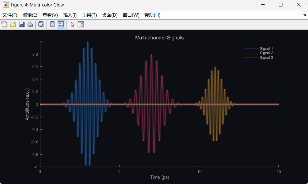
%  图3：深色背景 + 辉光效果（光子学演示风格）
%  ================================================================
fig3 = figure('Position', [150, 100, 700, 350], ...
              'Color', [0.05, 0.07, 0.1], ...
              'Name', 'Dark Background Glow Style');

ax3 = axes('Parent', fig3, 'Color', [0.05, 0.07, 0.1], ...
           'XColor', [0.6 0.6 0.6], 'YColor', [0.6 0.6 0.6], ...
           'GridColor', [0.2 0.2 0.2], 'GridAlpha', 0.5);
hold on;
grid on;

t3 = linspace(-5, 5, 5000);
envelope = exp(-t3.^2 / 2);
chirped  = envelope .* cos(2*pi*5*t3 + 1.5*t3.^2);

% 辉光层（从外到内：宽+透明 → 窄+实）
glow_widths = [5.0, 3.5, 2.5, 1.8, 1.2];
glow_alphas = [0.04, 0.07, 0.12, 0.20, 1.0];
glow_color  = [0.2, 0.8, 1.0];  % 青色辉光

for ii = 1:length(glow_widths)
    plot(t3, chirped, 'Color', [glow_color, glow_alphas(ii)], ...
         'LineWidth', glow_widths(ii));
end

% 包络线（虚线）
plot(t3, envelope,  '--', 'Color', [1 1 1 0.3], 'LineWidth', 0.6);
plot(t3, -envelope, '--', 'Color', [1 1 1 0.3], 'LineWidth', 0.6);

hold off;
xlabel('Time (ps)', 'Color', [0.7 0.7 0.7]);
ylabel('E-field (a.u.)', 'Color', [0.7 0.7 0.7]);
title('Chirped Optical Pulse', 'Color', [0.9 0.9 0.9], 'FontSize', 10);
xlim([-5 5]);
ylim([-1.3 1.3]);

set(fig3, 'InvertHardcopy', 'off');  % 保存时保留深色背景
print(fig3, 'NP_dark_glow', '-dpng', '-r300');
fprintf('✅ 深色风格图已保存: NP_dark_glow.png\n');

%% ================================================================
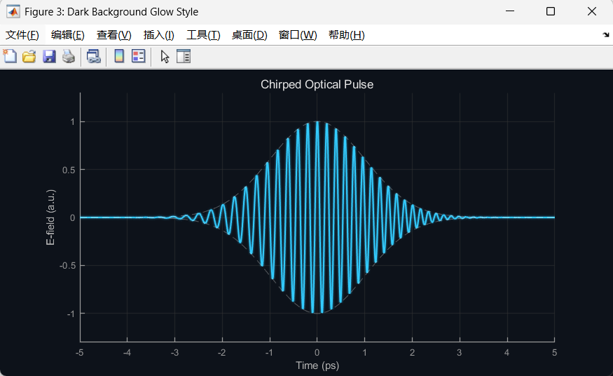
%  图4：深色背景多色辉光对比
%  ================================================================
fig4 = figure('Position', [200, 80, 800, 400], ...
              'Color', [0.05, 0.05, 0.08], ...
              'Name', 'Multi-color Glow');

ax4 = axes('Parent', fig4, 'Color', [0.05, 0.05, 0.08], ...
           'XColor', [0.5 0.5 0.5], 'YColor', [0.5 0.5 0.5]);
hold on;

t4 = linspace(0, 15, 4000);
signals = {
    exp(-(t4-3).^2/0.6) .* cos(2*pi*4*t4),       [0.2, 0.6, 1.0];   % 蓝
    exp(-(t4-7).^2/0.8) .* cos(2*pi*3*t4) * 0.8,  [1.0, 0.3, 0.5];   % 粉红
    exp(-(t4-11).^2/0.4) .* cos(2*pi*5*t4) * 0.6, [1.0, 0.7, 0.2];   % 琥珀
};

for ss = 1:size(signals, 1)
    sig = signals{ss, 1};
    clr = signals{ss, 2};
    % 辉光
    for jj = [5.0, 3.0, 1.8, 1.0]
        alpha_val = 0.03 + 0.15 * (1.0/jj);
        plot(t4, sig, 'Color', [clr, min(alpha_val, 1)], 'LineWidth', jj);
    end
end
hold off;

xlabel('Time (ps)', 'Color', [0.6 0.6 0.6]);
ylabel('Amplitude (a.u.)', 'Color', [0.6 0.6 0.6]);
title('Multi-channel Signals', 'Color', [0.85 0.85 0.85], 'FontSize', 10);
xlim([0 15]);
legend({'','','','Signal 1','','','','Signal 2','','','','Signal 3'}, ...
       'TextColor', [0.7 0.7 0.7], 'Color', 'none', 'Box', 'off', ...
       'FontSize', 7, 'Location', 'northeast');

set(fig4, 'InvertHardcopy', 'off');
print(fig4, 'NP_multi_glow', '-dpng', '-r300');
fprintf('✅ 多色辉光图已保存: NP_multi_glow.png\n');

fprintf('\n========== 全部完成 ==========\n');

%% ================================================================
%  局部函数定义 (放在文件末尾)
%  ================================================================

function cmap = nat_photonics_cmap()
% 自定义 Nature Photonics 风格 colormap (深蓝→青→白)
    n = 256;
    colors = [
        0.05, 0.05, 0.20;   % 深蓝
        0.00, 0.30, 0.60;   % 蓝
        0.00, 0.60, 0.60;   % 青
        0.20, 0.85, 0.60;   % 青绿
        0.95, 0.95, 0.80;   % 浅黄
        1.00, 0.60, 0.20;   % 橙
        0.85, 0.15, 0.15;   % 红
    ];
    x_orig = linspace(0, 1, size(colors, 1));
    x_new  = linspace(0, 1, n);
    cmap = interp1(x_orig, colors, x_new);
end

function pos = get_arrow_pos(ax, fig, x1, y1, x2, y2)
% 将数据坐标转换为 figure normalized 坐标，用于 annotation
    ax_pos = get(ax, 'Position');    % axes在figure中的位置
    xl = get(ax, 'XLim');
    yl = get(ax, 'YLim');
    
    % 数据 → axes normalized
    nx1 = (x1 - xl(1)) / (xl(2) - xl(1));
    ny1 = (y1 - yl(1)) / (yl(2) - yl(1));
    nx2 = (x2 - xl(1)) / (xl(2) - xl(1));
    ny2 = (y2 - yl(1)) / (yl(2) - yl(1));
    
    % axes normalized → figure normalized
    fx1 = ax_pos(1) + nx1 * ax_pos(3);
    fy1 = ax_pos(2) + ny1 * ax_pos(4);
    fx2 = ax_pos(1) + nx2 * ax_pos(3);
    fy2 = ax_pos(2) + ny2 * ax_pos(4);
    
    pos = [fx1, fy1, fx2-fx1, fy2-fy1];
end