1 背景
前面曾介绍过ILSVRC-2014比赛中的第二名VGG,本章将介绍当时的冠军GoogLeNet。谷歌研究团队于2014年发布论文 Going Deeper with Convolutions 讲述了该模型,其发表于CVPR (Conference on Computer Vision and Pattern Recognition, IEEE 计算机视觉与模式识别会议)。 从GoogLeNet模型名字也能看出,这是对LeNet经典模型的致敬。GoogLeNet借鉴了同年发表的模型即上一章介绍的NIN中的思想,并在此基础上进行了改进和创新,形成了前所未有的并行结构------ Inception 块**。**
2 原理
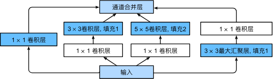
图1 Inception块的架构
Inception块的架构如书中图片所示,通过4个并行路径进行处理,注意这里和之前提到的所有多通道卷积层不同,Inception块中对每个路径处理过程的差异更大,并且每条路径上含有多个通道,最后利用一个通道合并层在通道维度上合并4条路径的输出结果。简单来说就是整个网络"变宽了"。
接下来我们仔细分析Inception块的结构,这是一个相当优雅的思路,输入数据会分别经过3种不同大小的卷积层和1个汇聚层产生4条路径的输出,每条输出都会再次经过下一个Inception块的4条路径处理,根据具排列组合我们可以知道,经过2次Inception块就会产生4*4=16条路径的处理结果,3次则产生64条,这些结果包含不同的卷积核大小,卷积和汇聚次数,利用有限的层数和参数极大的丰富了寻找不同深度的特征的路线。相比传统的单一卷积-汇聚路线,GoogLeNet更不依赖人工设置参数,能更加适应不同大小的图像特征,需要的参数和计算量也会更少。Inception块的提出可以说是CNN的又一次飞跃。
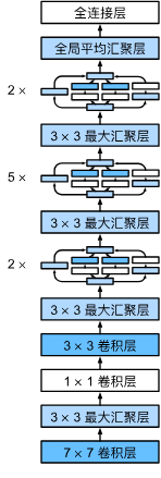
图2 GoogLeNet架构
GoogLeNet架构如图所示,其中Inception块的组合思想从VGG继承,用全局平局汇聚层代替展平的思想则与NIN一致。
3 实现
3.1 模型定义
下面的代码定义了一个Inception块,包含4条处理路径。c1-c4表示4条路径的输出通道数,其中第2、3条路径由于有两次卷积处理会产生两次输出,所以c2、c3用二元组表示。
python
import torch
from torch import nn
from torch.nn import functional as F
from d2l import torch as d2l


class Inception(nn.Module):
    # c1--c4是每条路径的输出通道数
    def __init__(self, in_channels, c1, c2, c3, c4, **kwargs):
        super(Inception, self).__init__(**kwargs)
        # 线路1,单1x1卷积层
        self.p1_1 = nn.Conv2d(in_channels, c1, kernel_size=1)
        # 线路2,1x1卷积层后接3x3卷积层
        self.p2_1 = nn.Conv2d(in_channels, c2[0], kernel_size=1)
        self.p2_2 = nn.Conv2d(c2[0], c2[1], kernel_size=3, padding=1)
        # 线路3,1x1卷积层后接5x5卷积层
        self.p3_1 = nn.Conv2d(in_channels, c3[0], kernel_size=1)
        self.p3_2 = nn.Conv2d(c3[0], c3[1], kernel_size=5, padding=2)
        # 线路4,3x3最大汇聚层后接1x1卷积层
        self.p4_1 = nn.MaxPool2d(kernel_size=3, stride=1, padding=1)
        self.p4_2 = nn.Conv2d(in_channels, c4, kernel_size=1)

    def forward(self, x):
        p1 = F.relu(self.p1_1(x))
        p2 = F.relu(self.p2_2(F.relu(self.p2_1(x))))
        p3 = F.relu(self.p3_2(F.relu(self.p3_1(x))))
        p4 = F.relu(self.p4_2(self.p4_1(x)))
        # 在通道维度上连结输出
        return torch.cat((p1, p2, p3, p4), dim=1)
下面的代码详细定义了GoogLeNet中每一个模块,如图2所示,以汇聚层划分模块,共划分出5个模块。
python
b1 = nn.Sequential(nn.Conv2d(1, 64, kernel_size=7, stride=2, padding=3),
                   nn.ReLU(),
                   nn.MaxPool2d(kernel_size=3, stride=2, padding=1))

b2 = nn.Sequential(nn.Conv2d(64, 64, kernel_size=1),
                   nn.ReLU(),
                   nn.Conv2d(64, 192, kernel_size=3, padding=1),
                   nn.ReLU(),
                   nn.MaxPool2d(kernel_size=3, stride=2, padding=1))

b3 = nn.Sequential(Inception(192, 64, (96, 128), (16, 32), 32),
                   Inception(256, 128, (128, 192), (32, 96), 64),
                   nn.MaxPool2d(kernel_size=3, stride=2, padding=1))

b4 = nn.Sequential(Inception(480, 192, (96, 208), (16, 48), 64),
                   Inception(512, 160, (112, 224), (24, 64), 64),
                   Inception(512, 128, (128, 256), (24, 64), 64),
                   Inception(512, 112, (144, 288), (32, 64), 64),
                   Inception(528, 256, (160, 320), (32, 128), 128),
                   nn.MaxPool2d(kernel_size=3, stride=2, padding=1))

b5 = nn.Sequential(Inception(832, 256, (160, 320), (32, 128), 128),
                   Inception(832, 384, (192, 384), (48, 128), 128),
                   nn.AdaptiveAvgPool2d((1,1)),
                   nn.Flatten())

net = nn.Sequential(b1, b2, b3, b4, b5, nn.Linear(1024, 10))
下面的代码展示了各模块的输出形状。
python
X = torch.rand(size=(1, 1, 96, 96))
for layer in net:
    X = layer(X)
    print(layer.__class__.__name__,'output shape:\t', X.shape)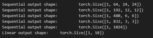
3.2 模型训练
为了减少计算量,Fashion-MNIST数据集之前将图像宽度和高度从224降低至96。
python
lr, num_epochs, batch_size = 0.1, 10, 128
train_iter, test_iter = d2l.load_data_fashion_mnist(batch_size, resize=96)
d2l.train_ch6(net, train_iter, test_iter, num_epochs, lr, d2l.try_gpu())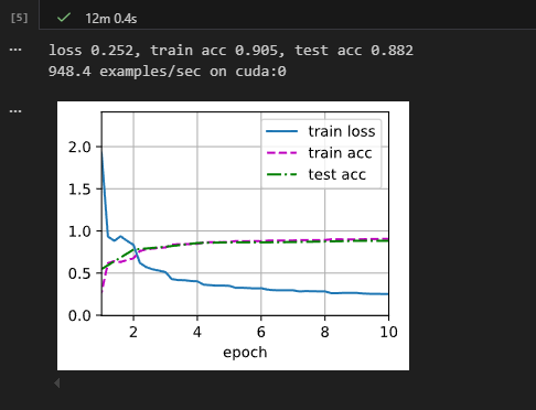
参考文献
1《动手学深度学习》,https://zh-v2.d2l.ai/