【大模型】大模型学习总结之机器学习-3.模型评估

这里写目录标题

• 什么是模型评估和模型选择？
• 损失函数
• 经验误差
• 欠拟合和过拟合
• • demo
• 正则化
• • demo
• 交叉验证

什么是模型评估和模型选择？

• 模型评估：是判断模型在特定数据上的表现能力，核心是回答"这个模型好不好"；
• 模型选择：则是在多个候选模型中挑选最优者，核心是回答"哪个模型更好"。

两者的本质区别在于：

评估关注单一模型的性能度量（如准确率、F1分数）

选择关注不同模型间的性能比较与权衡

实践中的核心矛盾：我们无法获得真实误差（在所有可能数据上的期望误差），只能基于有限样本进行估计。这就引出了经验误差的概念。

损失函数

衡量预测错误的标尺, 度量模型的好坏。

损失函数定义了单个预测的"代价"程度，是模型优化的基础。损失函数是非负数。

损失函数	适用场景	核心特点
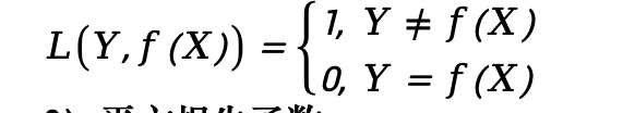
0-1损失	分类问题	预测正确为0，错误为1；不可导，理论分析用
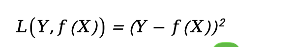
平方损失	回归问题	(y-ŷ)²；对异常值敏感，可导
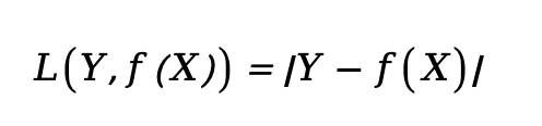
绝对损失	回归问题 |y-ŷ|；鲁棒性强，不可导
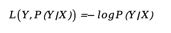
对数损失	概率估计	-logP(y|x)；适合概率分类
Hinge损失	SVM	max(0, 1-yf(x))；适合间隔最大化

• 0-1损失
  

• 平方损失
  

• 绝对损失
  

• 对数损失 *
  

• Hinge损失

关键洞察：损失函数的选择直接决定了模型的优化目标和敏感度。例如，平方损失对异常值敏感，而绝对损失则更稳健。

经验误差

有限样本的无奈近似，就是训练误差 ，损失误差指的是单个样本、经验误差指的是所有数据。

给定一个训练数据集，数据个数为n：

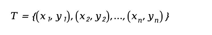
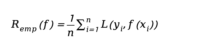
根据选取的损失函数，就可以计算出模型f(X)在训练集上的平均误差，称为训练误差，也被称作 经验误差（empirical error） 或 经验风险（empirical risk）。

类似地，在测试数据集上平均误差，被称为测试误差或者 泛化误差（generalization error）。

一般情况下对模型评估的策略，就是考察经验误差；当经验风险最小时，就认为取到了最优的模型。这种策略被称为 经验风险最小化（empirical risk minimization，ERM）。

经验误差（训练误差）是模型在训练集上的平均损失。由于数据有限，它只是真实误差的一个估计，且存在以下关键问题：

• 估计偏差：训练集可能不代表真实分布
• 过拟合风险：经验误差低≠泛化能力强
• 样本依赖：不同训练集会得到不同经验误差

这解释了为什么不能仅用训练误差来评估模型，也引出了欠拟合和过拟合的讨论。

欠拟合和过拟合

这是模型复杂度与数据复杂度不匹配的表现：

拟合（Fitting）是指机器学习模型在训练数据上学习到规律并生成预测结果的过程。理想情况下，模型能够准确地捕捉训练数据的模式，并且在未见过的新数据（测试数据）上也有良好的表现；即模型具有良好的 泛化能力。

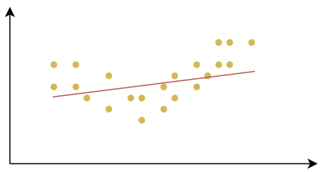
欠拟合（Underfitting）：是指模型在训练数据上表现不佳，无法很好地捕捉数据中的规律。这样的模型不仅在训练集上表现不好，在测试集上也同样表现差。

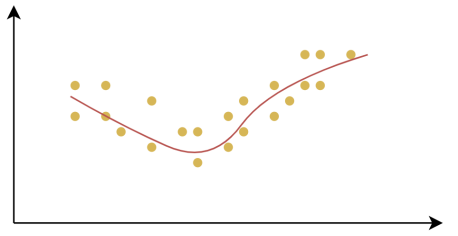
过拟合（Overfitting）：是指模型在训练数据上表现得很好，但在测试数据或新数据上表现较差的情况。过拟合的模型对训练数据中的噪声或细节过度敏感，把训练样本自身的一些特点当作了所有潜在样本都会具有的一般性质，从而失去了泛化能力。

产生欠拟合和过拟合的根本原因，是模型的复杂度过低或过高，从而导致测试误差（泛化误差）偏大。

• 欠拟合（高偏差）：

  • 现象：训练误差高，测试误差也高
  • 原因：模型过于简单，无法捕捉数据模式
  • 解决：增加模型复杂度（更多特征、更深网络）

• 过拟合（高方差）：

  • 现象：训练误差低，测试误差高
  • 原因：模型过于复杂，记住了训练噪声
  • 解决：正则化、更多数据、特征选择、早停

直观理解：想象你在学习一门课程，欠拟合是"没学会"，过拟合是"死记硬背但不会应用"。

demo

# bias_variance_demo.py
import numpy as np
import matplotlib.pyplot as plt
from sklearn.model_selection import train_test_split
from sklearn.linear_model import LinearRegression
from sklearn.metrics import mean_squared_error, r2_score
from sklearn.preprocessing import PolynomialFeatures
from sklearn.pipeline import Pipeline

# 设置中文字体和负号显示
plt.rcParams["font.sans-serif"] = ["SimHei", "KaiTi", "Arial Unicode MS"]
plt.rcParams["axes.unicode_minus"] = False

# 设置随机种子保证可重复性
np.random.seed(42)

# 生成模拟数据（正弦函数+噪声）
def generate_data(n_samples=300, noise_level=0.3):
    """生成带有噪声的正弦函数数据"""
    X = np.linspace(-3, 3, n_samples).reshape(-1, 1)
    # 真实函数：y = sin(x) + 噪声
    y_true = np.sin(X)
    y = y_true + np.random.normal(0, noise_level, n_samples).reshape(-1, 1)
    return X, y, y_true

# 创建多项式回归模型
def create_polynomial_model(degree):
    """创建指定阶数的多项式回归模型"""
    model = Pipeline([
        ('poly', PolynomialFeatures(degree=degree)),
        ('linear', LinearRegression())
    ])
    return model

# 评估模型性能
def evaluate_model(model, X_train, X_test, y_train, y_test):
    """评估模型在训练集和测试集上的性能"""
    # 训练集评估
    y_train_pred = model.predict(X_train)
    train_mse = mean_squared_error(y_train, y_train_pred)
    train_r2 = r2_score(y_train, y_train_pred)

    # 测试集评估
    y_test_pred = model.predict(X_test)
    test_mse = mean_squared_error(y_test, y_test_pred)
    test_r2 = r2_score(y_test, y_test_pred)

    return {
        'train_mse': train_mse,
        'train_r2': train_r2,
        'test_mse': test_mse,
        'test_r2': test_r2,
        'y_train_pred': y_train_pred,
        'y_test_pred': y_test_pred
    }

# 主函数
def main():
    # 生成数据
    X, y, y_true = generate_data(n_samples=300, noise_level=0.3)

    # 划分训练集和测试集
    X_train, X_test, y_train, y_test = train_test_split(
        X, y, test_size=0.2, random_state=42
    )

    # 定义三种不同复杂度的模型
    models_config = [
        {'degree': 1, 'title': '欠拟合 (线性模型)', 'color': 'blue', 'linestyle': '--'},
        {'degree': 5, 'title': '恰当拟合 (5阶多项式)', 'color': 'green', 'linestyle': '-'},
        {'degree': 15, 'title': '过拟合 (15阶多项式)', 'color': 'red', 'linestyle': '-'}
    ]

    # 创建图表
    fig, axes = plt.subplots(2, 3, figsize=(18, 10))
    fig.suptitle('欠拟合 vs 恰当拟合 vs 过拟合：模型复杂度与泛化能力', fontsize=16, fontweight='bold')

    # 第一行：数据拟合对比
    for idx, config in enumerate(models_config):
        ax = axes[0, idx]

        # 训练模型
        model = create_polynomial_model(config['degree'])
        model.fit(X_train, y_train)

        # 评估模型
        metrics = evaluate_model(model, X_train, X_test, y_train, y_test)

        # 生成平滑的预测曲线
        X_smooth = np.linspace(-3, 3, 200).reshape(-1, 1)
        y_smooth_pred = model.predict(X_smooth)

        # 绘制真实函数曲线
        y_smooth_true = np.sin(X_smooth)
        ax.plot(X_smooth, y_smooth_true, 'k-', linewidth=2, alpha=0.6, label='真实函数')

        # 绘制训练数据点
        ax.scatter(X_train, y_train, c='lightblue', alpha=0.6, s=30, label='训练数据')

        # 绘制测试数据点
        ax.scatter(X_test, y_test, c='orange', alpha=0.8, s=30, label='测试数据')

        # 绘制模型预测曲线
        ax.plot(X_smooth, y_smooth_pred,
                color=config['color'],
                linestyle=config['linestyle'],
                linewidth=3,
                label=config['title'])

        # 设置标题和标签
        ax.set_title(f'{config["title"]}', fontsize=12, fontweight='bold')
        ax.set_xlabel('X', fontsize=10)
        ax.set_ylabel('Y', fontsize=10)
        ax.legend(loc='upper right', fontsize=8)
        ax.grid(True, alpha=0.3)

        # 在图表上显示性能指标
        textstr = f'训练集 MSE: {metrics["train_mse"]:.4f}\n'
        textstr += f'测试集 MSE: {metrics["test_mse"]:.4f}\n'
        textstr += f'训练集 R²: {metrics["train_r2"]:.4f}\n'
        textstr += f'测试集 R²: {metrics["test_r2"]:.4f}'

        props = dict(boxstyle='round', facecolor='wheat', alpha=0.8)
        ax.text(0.05, 0.95, textstr, transform=ax.transAxes, fontsize=9,
                verticalalignment='top', bbox=props)

    # 第二行：学习曲线分析
    degrees = range(1, 18)
    train_mses = []
    test_mses = []

    for degree in degrees:
        model = create_polynomial_model(degree)
        model.fit(X_train, y_train)
        metrics = evaluate_model(model, X_train, X_test, y_train, y_test)
        train_mses.append(metrics['train_mse'])
        test_mses.append(metrics['test_mse'])

    # 绘制学习曲线
    ax = axes[1, :]
    ax = axes[1, 0]  # 使用第一个子图
    ax.plot(degrees, train_mses, 'b-o', linewidth=2, markersize=4, label='训练集误差')
    ax.plot(degrees, test_mses, 'r-s', linewidth=2, markersize=4, label='测试集误差')
    ax.axvline(x=5, color='green', linestyle='--', alpha=0.7, label='最优复杂度(度=5)')

    # 标注区域
    ax.axvspan(1, 3, alpha=0.2, color='blue', label='欠拟合区域')
    ax.axvspan(4, 8, alpha=0.2, color='green', label='恰当拟合区域')
    ax.axvspan(9, 17, alpha=0.2, color='red', label='过拟合区域')

    ax.set_xlabel('多项式阶数 (模型复杂度)', fontsize=12)
    ax.set_ylabel('均方误差 (MSE)', fontsize=12)
    ax.set_title('模型复杂度与误差的关系', fontsize=12, fontweight='bold')
    ax.legend(loc='upper right', fontsize=9)
    ax.grid(True, alpha=0.3)

    # 隐藏另外两个子图
    axes[1, 1].axis('off')
    axes[1, 2].axis('off')

    # 添加总结性文字
    summary_text = """
    关键观察：
    1. 欠拟合：训练集和测试集误差都很高，模型太简单无法捕捉数据模式
    2. 恰当拟合：训练集误差较低，测试集误差也较低，泛化能力强
    3. 过拟合：训练集误差很低，但测试集误差很高，模型记住了噪声

    实践建议：
    • 选择训练集和测试集误差都较低且接近的模型
    • 关注验证集误差（或测试集误差）的最小值
    • 避免选择训练集误差持续下降但测试集误差开始上升的模型
    """

    axes[1, 1].text(0.1, 0.5, summary_text, fontsize=11, verticalalignment='center',
                    bbox=dict(boxstyle='round', facecolor='lightyellow', alpha=0.8))

    # 添加数学公式说明
    formula_text = """
    数学原理：

    偏差-方差权衡：

    期望误差 = 偏差² + 方差 + 不可约误差

    • 欠拟合：高偏差，低方差
    • 过拟合：低偏差，高方差
    • 恰当拟合：偏差和方差平衡

    正则化可帮助控制模型复杂度，
    在偏差和方差间找到最佳平衡点。
    """

    axes[1, 2].text(0.1, 0.5, formula_text, fontsize=10, verticalalignment='center',
                    bbox=dict(boxstyle='round', facecolor='lightblue', alpha=0.8))

    plt.tight_layout()
    plt.savefig('bias_variance_analysis.png', dpi=300, bbox_inches='tight')
    plt.show()

    # 打印详细的数值分析
    print("=" * 60)
    print("模型性能详细分析")
    print("=" * 60)

    for config in models_config:
        model = create_polynomial_model(config['degree'])
        model.fit(X_train, y_train)
        metrics = evaluate_model(model, X_train, X_test, y_train, y_test)

        print(f"\n{config['title']}")
        print("-" * 40)
        print(f"训练集 MSE: {metrics['train_mse']:.6f}")
        print(f"测试集 MSE: {metrics['test_mse']:.6f}")
        print(f"训练集 R²: {metrics['train_r2']:.6f}")
        print(f"测试集 R²: {metrics['test_r2']:.6f}")
        print(f"泛化差距: {abs(metrics['train_mse'] - metrics['test_mse']):.6f}")

    print("\n" + "=" * 60)
    print("最优模型选择建议")
    print("=" * 60)

    # 找到测试集误差最小的模型
    best_degree_idx = np.argmin(test_mses)
    best_degree = degrees[best_degree_idx]
    print(f"最优多项式阶数: {best_degree}")
    print(f"最小测试集误差: {test_mses[best_degree_idx]:.6f}")
    print(f"对应训练集误差: {train_mses[best_degree_idx]:.6f}")

if __name__ == "__main__":
    main()

运行结果

===========================================================
模型性能详细分析
============================================================

欠拟合 (线性模型)
----------------------------------------
训练集 MSE: 0.256397
测试集 MSE: 0.264323
训练集 R²: 0.587686
测试集 R²: 0.611585
泛化差距: 0.007926

恰当拟合 (5阶多项式)
----------------------------------------
训练集 MSE: 0.092532
测试集 MSE: 0.061183
训练集 R²: 0.851199
测试集 R²: 0.910093
泛化差距: 0.031349

过拟合 (15阶多项式)
----------------------------------------
训练集 MSE: 0.089134
测试集 MSE: 0.065085
训练集 R²: 0.856663
测试集 R²: 0.904359
泛化差距: 0.024048

============================================================
最优模型选择建议
============================================================
最优多项式阶数: 4
最小测试集误差: 0.056396
对应训练集误差: 0.097730

Process finished with exit code 0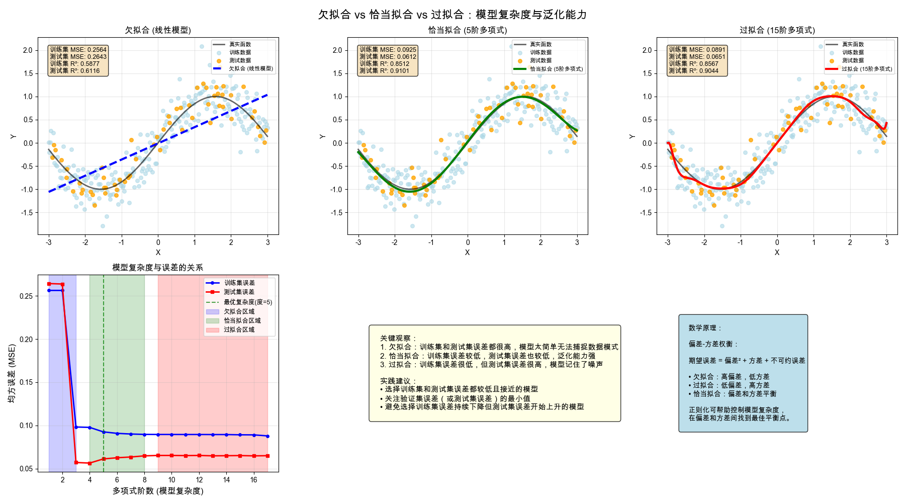

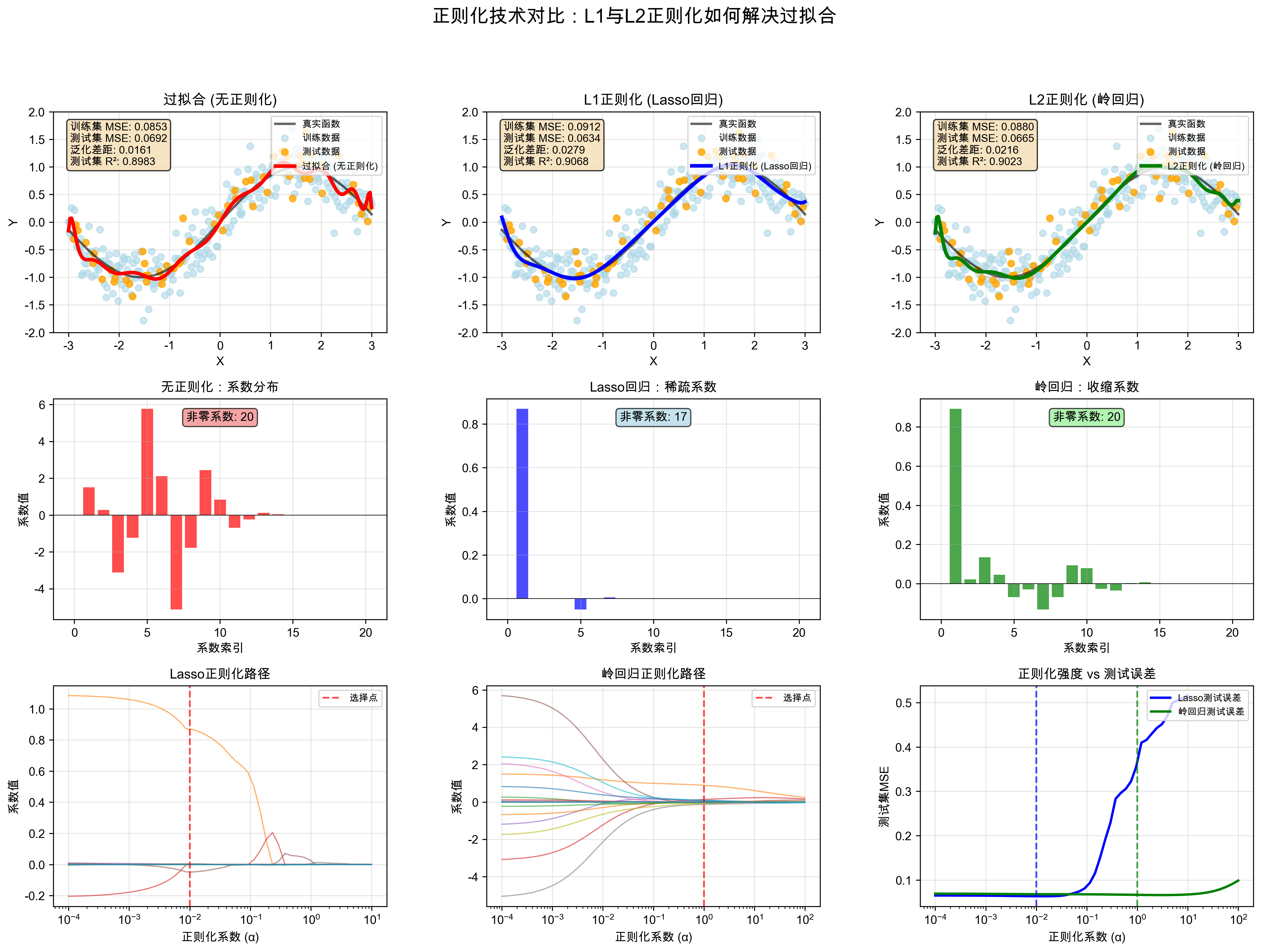
正则化

正则化通过在损失函数中加入约束项，防止模型过拟合：

L1正则化（Lasso）：

• 约束项：λ∑|w|
• 效果：产生稀疏解，自动特征选择
• 适用：高维数据、特征筛选

L2正则化（Ridge）：

• 约束项：λ∑w²
• 效果：权重平滑，防止某个特征主导
• 适用：共线性问题、防止过拟合

Elastic Net：

• 结合L1+L2：λ₁∑|w| + λ₂∑w²
• 兼顾稀疏性和平滑性

核心思想：正则化是对模型复杂度的"惩罚"，迫使模型学习更简单的模式，提升泛化能力。

demo

#!/usr/bin/env python
# -*- coding: utf-8 -*-
"""
@Date          : 2026/3/23
@File          : 1.py
@Author        : liwei68
@Description   : 
"""

import numpy as np
import matplotlib.pyplot as plt
from sklearn.model_selection import train_test_split, cross_val_score
from sklearn.linear_model import LinearRegression, Lasso, Ridge
from sklearn.metrics import mean_squared_error, r2_score
from sklearn.preprocessing import PolynomialFeatures
from sklearn.pipeline import Pipeline

# 设置中文字体和负号显示
plt.rcParams["font.sans-serif"] = ["SimHei", "KaiTi", "Arial Unicode MS"]
plt.rcParams["axes.unicode_minus"] = False

# 设置随机种子保证可重复性
np.random.seed(42)

# 生成模拟数据（正弦函数+噪声）
def generate_data(n_samples=300, noise_level=0.3):
    """生成带有噪声的正弦函数数据"""
    X = np.linspace(-3, 3, n_samples).reshape(-1, 1)
    # 真实函数：y = sin(x) + 噪声
    y_true = np.sin(X)
    y = y_true + np.random.normal(0, noise_level, n_samples).reshape(-1, 1)
    return X, y, y_true

# 创建多项式回归模型
def create_polynomial_model(degree, regularization=None, alpha=1.0):
    """创建多项式回归模型，支持不同的正则化方法"""
    if regularization == 'lasso':
        model = Pipeline([
            ('poly', PolynomialFeatures(degree=degree)),
            ('linear', Lasso(alpha=alpha, max_iter=10000, random_state=42))
        ])
    elif regularization == 'ridge':
        model = Pipeline([
            ('poly', PolynomialFeatures(degree=degree)),
            ('linear', Ridge(alpha=alpha, random_state=42))
        ])
    else:
        model = Pipeline([
            ('poly', PolynomialFeatures(degree=degree)),
            ('linear', LinearRegression())
        ])
    return model

# 评估模型性能
def evaluate_model(model, X_train, X_test, y_train, y_test):
    """评估模型在训练集和测试集上的性能"""
    # 训练集评估
    y_train_pred = model.predict(X_train)
    train_mse = mean_squared_error(y_train, y_train_pred)
    train_r2 = r2_score(y_train, y_train_pred)

    # 测试集评估
    y_test_pred = model.predict(X_test)
    test_mse = mean_squared_error(y_test, y_test_pred)
    test_r2 = r2_score(y_test, y_test_pred)

    return {
        'train_mse': train_mse,
        'train_r2': train_r2,
        'test_mse': test_mse,
        'test_r2': test_r2,
        'y_train_pred': y_train_pred,
        'y_test_pred': y_test_pred
    }

def main():
    # 生成数据
    X, y, y_true = generate_data(n_samples=300, noise_level=0.3)

    # 划分训练集和测试集
    X_train, X_test, y_train, y_test = train_test_split(
        X, y, test_size=0.2, random_state=42
    )

    # 定义不同的正则化方法
    models_config = [
        {
            'regularization': None,
            'alpha': None,
            'title': '过拟合 (无正则化)',
            'color': 'red',
            'linestyle': '-'
        },
        {
            'regularization': 'lasso',
            'alpha': 0.01,
            'title': 'L1正则化 (Lasso回归)',
            'color': 'blue',
            'linestyle': '-'
        },
        {
            'regularization': 'ridge',
            'alpha': 1.0,
            'title': 'L2正则化 (岭回归)',
            'color': 'green',
            'linestyle': '-'
        }
    ]

    # 创建图表
    fig = plt.figure(figsize=(18, 12))
    gs = fig.add_gridspec(3, 3, hspace=0.3, wspace=0.3)

    # 第一行：拟合效果对比
    for idx, config in enumerate(models_config):
        ax = fig.add_subplot(gs[0, idx])

        # 训练模型
        model = create_polynomial_model(degree=20,
                                       regularization=config['regularization'],
                                       alpha=config['alpha'])
        model.fit(X_train, y_train)

        # 评估模型
        metrics = evaluate_model(model, X_train, X_test, y_train, y_test)

        # 生成平滑的预测曲线
        X_smooth = np.linspace(-3, 3, 200).reshape(-1, 1)
        y_smooth_pred = model.predict(X_smooth)

        # 绘制真实函数曲线
        y_smooth_true = np.sin(X_smooth)
        ax.plot(X_smooth, y_smooth_true, 'k-', linewidth=2, alpha=0.6, label='真实函数')

        # 绘制训练数据点
        ax.scatter(X_train, y_train, c='lightblue', alpha=0.6, s=30, label='训练数据')

        # 绘制测试数据点
        ax.scatter(X_test, y_test, c='orange', alpha=0.8, s=30, label='测试数据')

        # 绘制模型预测曲线
        ax.plot(X_smooth, y_smooth_pred,
                color=config['color'],
                linestyle=config['linestyle'],
                linewidth=3,
                label=config['title'])

        # 设置标题和标签
        ax.set_title(f'{config["title"]}', fontsize=12, fontweight='bold')
        ax.set_xlabel('X', fontsize=10)
        ax.set_ylabel('Y', fontsize=10)
        ax.legend(loc='upper right', fontsize=8)
        ax.grid(True, alpha=0.3)
        ax.set_ylim(-2, 2)

        # 在图表上显示性能指标
        textstr = f'训练集 MSE: {metrics["train_mse"]:.4f}\n'
        textstr += f'测试集 MSE: {metrics["test_mse"]:.4f}\n'
        textstr += f'泛化差距: {abs(metrics["train_mse"] - metrics["test_mse"]):.4f}\n'
        textstr += f'测试集 R²: {metrics["test_r2"]:.4f}'

        props = dict(boxstyle='round', facecolor='wheat', alpha=0.8)
        ax.text(0.05, 0.95, textstr, transform=ax.transAxes, fontsize=9,
                verticalalignment='top', bbox=props)

        # 保存模型系数用于后续分析
        if config['regularization'] is None:
            linear_coefs = model.named_steps['linear'].coef_.flatten()
        elif config['regularization'] == 'lasso':
            lasso_coefs = model.named_steps['linear'].coef_.flatten()
        elif config['regularization'] == 'ridge':
            ridge_coefs = model.named_steps['linear'].coef_.flatten()

    # 第二行：系数对比
    # 绘制无正则化的系数
    ax1 = fig.add_subplot(gs[1, 0])
    ax1.bar(np.arange(len(linear_coefs)), linear_coefs, color='red', alpha=0.7)
    ax1.axhline(y=0, color='k', linestyle='-', linewidth=0.5)
    ax1.set_xlabel('系数索引', fontsize=10)
    ax1.set_ylabel('系数值', fontsize=10)
    ax1.set_title('无正则化：系数分布', fontsize=11, fontweight='bold')
    ax1.grid(True, alpha=0.3)
    ax1.text(0.5, 0.9, f'非零系数: {np.sum(linear_coefs != 0)}',
             transform=ax1.transAxes, ha='center', fontsize=10,
             bbox=dict(boxstyle='round', facecolor='lightcoral', alpha=0.7))

    # 绘制Lasso回归的系数
    ax2 = fig.add_subplot(gs[1, 1])
    ax2.bar(np.arange(len(lasso_coefs)), lasso_coefs, color='blue', alpha=0.7)
    ax2.axhline(y=0, color='k', linestyle='-', linewidth=0.5)
    ax2.set_xlabel('系数索引', fontsize=10)
    ax2.set_ylabel('系数值', fontsize=10)
    ax2.set_title('Lasso回归：稀疏系数', fontsize=11, fontweight='bold')
    ax2.grid(True, alpha=0.3)
    ax2.text(0.5, 0.9, f'非零系数: {np.sum(lasso_coefs != 0)}',
             transform=ax2.transAxes, ha='center', fontsize=10,
             bbox=dict(boxstyle='round', facecolor='lightblue', alpha=0.7))

    # 绘制岭回归的系数
    ax3 = fig.add_subplot(gs[1, 2])
    ax3.bar(np.arange(len(ridge_coefs)), ridge_coefs, color='green', alpha=0.7)
    ax3.axhline(y=0, color='k', linestyle='-', linewidth=0.5)
    ax3.set_xlabel('系数索引', fontsize=10)
    ax3.set_ylabel('系数值', fontsize=10)
    ax3.set_title('岭回归：收缩系数', fontsize=11, fontweight='bold')
    ax3.grid(True, alpha=0.3)
    ax3.text(0.5, 0.9, f'非零系数: {np.sum(ridge_coefs != 0)}',
             transform=ax3.transAxes, ha='center', fontsize=10,
             bbox=dict(boxstyle='round', facecolor='lightgreen', alpha=0.7))

    # 第三行：正则化强度分析
    # Lasso正则化路径
    ax4 = fig.add_subplot(gs[2, 0])
    alphas_lasso = np.logspace(-4, 1, 50)
    coefs_lasso = []
    test_errors_lasso = []

    for alpha in alphas_lasso:
        model = create_polynomial_model(degree=20, regularization='lasso', alpha=alpha)
        model.fit(X_train, y_train)
        coefs_lasso.append(model.named_steps['linear'].coef_.flatten())

        # 计算测试误差
        y_pred = model.predict(X_test)
        test_errors_lasso.append(mean_squared_error(y_test, y_pred))

    coefs_lasso = np.array(coefs_lasso)

    # 绘制正则化路径
    for i in range(coefs_lasso.shape[1]):
        ax4.plot(alphas_lasso, coefs_lasso[:, i], linewidth=1, alpha=0.6)

    ax4.set_xscale('log')
    ax4.set_xlabel('正则化系数 (α)', fontsize=10)
    ax4.set_ylabel('系数值', fontsize=10)
    ax4.set_title('Lasso正则化路径', fontsize=11, fontweight='bold')
    ax4.grid(True, alpha=0.3)
    ax4.axvline(x=0.01, color='red', linestyle='--', alpha=0.7, label='选择点')
    ax4.legend(loc='upper right', fontsize=8)

    # 岭回归正则化路径
    ax5 = fig.add_subplot(gs[2, 1])
    alphas_ridge = np.logspace(-4, 2, 50)
    coefs_ridge = []
    test_errors_ridge = []

    for alpha in alphas_ridge:
        model = create_polynomial_model(degree=20, regularization='ridge', alpha=alpha)
        model.fit(X_train, y_train)
        coefs_ridge.append(model.named_steps['linear'].coef_.flatten())

        # 计算测试误差
        y_pred = model.predict(X_test)
        test_errors_ridge.append(mean_squared_error(y_test, y_pred))

    coefs_ridge = np.array(coefs_ridge)

    # 绘制正则化路径
    for i in range(coefs_ridge.shape[1]):
        ax5.plot(alphas_ridge, coefs_ridge[:, i], linewidth=1, alpha=0.6)

    ax5.set_xscale('log')
    ax5.set_xlabel('正则化系数 (α)', fontsize=10)
    ax5.set_ylabel('系数值', fontsize=10)
    ax5.set_title('岭回归正则化路径', fontsize=11, fontweight='bold')
    ax5.grid(True, alpha=0.3)
    ax5.axvline(x=1.0, color='red', linestyle='--', alpha=0.7, label='选择点')
    ax5.legend(loc='upper right', fontsize=8)

    # 测试误差对比
    ax6 = fig.add_subplot(gs[2, 2])
    ax6.plot(alphas_lasso, test_errors_lasso, 'b-', linewidth=2, label='Lasso测试误差')
    ax6.plot(alphas_ridge, test_errors_ridge, 'g-', linewidth=2, label='岭回归测试误差')
    ax6.set_xscale('log')
    ax6.set_xlabel('正则化系数 (α)', fontsize=10)
    ax6.set_ylabel('测试集MSE', fontsize=10)
    ax6.set_title('正则化强度 vs 测试误差', fontsize=11, fontweight='bold')
    ax6.grid(True, alpha=0.3)
    ax6.axvline(x=0.01, color='blue', linestyle='--', alpha=0.7)
    ax6.axvline(x=1.0, color='green', linestyle='--', alpha=0.7)
    ax6.legend(loc='upper right', fontsize=8)

    plt.suptitle('正则化技术对比：L1与L2正则化如何解决过拟合', fontsize=16, fontweight='bold')
    plt.savefig('regularization_analysis.png', dpi=300, bbox_inches='tight')
    plt.show()

    # 打印详细的数值分析
    print("=" * 70)
    print("正则化效果详细分析")
    print("=" * 70)

    for config in models_config:
        model = create_polynomial_model(degree=20,
                                       regularization=config['regularization'],
                                       alpha=config['alpha'])
        model.fit(X_train, y_train)
        metrics = evaluate_model(model, X_train, X_test, y_train, y_test)

        coefs = model.named_steps['linear'].coef_

        print(f"\n{config['title']}")
        print("-" * 50)
        print(f"训练集 MSE: {metrics['train_mse']:.6f}")
        print(f"测试集 MSE: {metrics['test_mse']:.6f}")
        print(f"泛化差距: {abs(metrics['train_mse'] - metrics['test_mse']):.6f}")
        print(f"测试集 R²: {metrics['test_r2']:.6f}")
        print(f"非零系数数量: {np.sum(coefs != 0)}")
        print(f"系数绝对值均值: {np.mean(np.abs(coefs)):.6f}")
        print(f"系数绝对值最大值: {np.max(np.abs(coefs)):.6f}")

    print("\n" + "=" * 70)
    print("正则化强度与模型性能关系分析")
    print("=" * 70)

    # 找到最优的正则化参数
    best_lasso_idx = np.argmin(test_errors_lasso)
    best_ridge_idx = np.argmin(test_errors_ridge)

    print(f"\nLasso最优参数:")
    print(f"最优 α: {alphas_lasso[best_lasso_idx]:.6f}")
    print(f"最小测试误差: {test_errors_lasso[best_lasso_idx]:.6f}")

    print(f"\n岭回归最优参数:")
    print(f"最优 α: {alphas_ridge[best_ridge_idx]:.6f}")
    print(f"最小测试误差: {test_errors_ridge[best_ridge_idx]:.6f}")

    print("\n" + "=" * 70)
    print("正则化效果总结")
    print("=" * 70)
    print("""
    1. L1正则化 (Lasso):
       - 特点：产生稀疏解，许多系数变为0
       - 优势：自动特征选择，模型可解释性强
       - 适用：高维数据、特征选择场景

    2. L2正则化 (岭回归):
       - 特点：所有系数都收缩但不为零
       - 优势：数值稳定性好，处理共线性问题
       - 适用：大多数回归问题、特征间相关性高

    3. 正则化参数选择：
       - α过小：正则化效果弱，仍可能过拟合
       - α过大：正则化效果强，可能导致欠拟合
       - 建议通过交叉验证选择最优α值

    4. 实践建议：
       - 优先尝试L2正则化，效果通常更稳定
       - 需要特征选择时使用L1正则化
       - 可以考虑Elastic Net结合L1和L2的优势
    """)

if __name__ == "__main__":
    main()

运行结果

交叉验证

为了解决单次划分的偶然性，交叉验证提供了更稳健的评估方法：

k折交叉验证：

• 将数据分成k份，轮流用k-1份训练，1份验证
• 重复k次，取平均性能
• 常用k=5或k=10

留一法（LOOCV）：

• k=n的特殊情况，每次留1个样本验证
• 评估最准确但计算成本高

分层k折：

• 保持每折的类别比例
• 适用于不平衡数据集

时间序列交叉验证：

• 按时间顺序划分，避免未来信息泄露
• 适用于时序数据

实践建议：

• 小数据集：使用k折交叉验证（k=5或10）
• 大数据集：可用简单的训练-验证-测试集划分
• 模型选择：在验证集上调整超参数，测试集仅用于最终评估