catalogue
- 数据操作基础
- 数据读写
- 数据抽样
- 缺失值处理、重复值处理
- plotly绘图
- ggplot2绘图
- 课内实训:医疗保费预测
- 餐饮企业客户价值分析
- 航空公司客户价值分析
- 课内实训:通信企业客户流失预测
- 杭州二手房数据预处理
- 模型参数优化
- 期中编程题
- 期末复习(二)
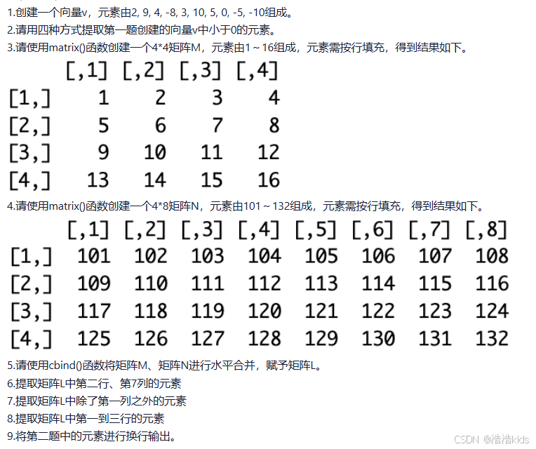
数据操作基础
r
#第一题
v <- c(2,9,4,-8,3,10,5,0,-5,-10)

#第二题
#方法一
for (i in v) {
  if(i < 0)
    cat(i," ")
}
#方法二
print(v[v < 0])
#方法三
print(v[which(v < 0)])
#方法四
print(subset(v,v < 0))

#第三题
M <- matrix(c(1:16),nrow = 4,ncol = 4,byrow = TRUE)
print(M)

#第四题
N <- matrix(c(101:132),nrow = 4,ncol = 8,byrow = TRUE)
print(N)

#第五题
L <- cbind(M,N)
print(L)

#第六题
print(L[2,7])

#第七题
print(L[,-1])

#第八题
print(L[c(1:3),])

#第九题
for (i in v) {
  if(i < 0)
    print(i)
}
数据读写

r
#第一题
iris <- read.csv("iris.csv",encoding = "UTF-8")
print(iris)

#第二题
scaled <- scale(iris[,4],center = TRUE,scale = TRUE)
print(scaled)

#第三题
write.csv(scaled,"iris_scale.csv",row.names = FALSE)
newdata <- read.csv("iris_scale.csv")
print(newdata)

#第四题
data <- read.xlsx("餐饮企业客户价值分析.xls",sheetIndex = 1)
print(data)

#第五题
data <- subset(data,select = -Id)

#第六题
write.csv(data,"RFM.csv",row.names = FALSE)
数据抽样

r
iris <- read.csv("iris.csv",encoding = "UTF-8")
print(iris)
print(iris[,c(1:4)])
print(iris[,5])
set.seed(123)
train_index <- sample(1:nrow(iris),size = round(0.8 * nrow(iris)))
train_iris <- iris[train_index,] #训练集
test_iris <- iris[-train_index,] #测试集
print(train_iris)
print(test_iris)
先下载select()所在的包:install.packages("dplyr",repos = "https://mirrors.ustc.edu.cn/CRAN/")
r
data <- read.csv("二手车(已处理缺失值、重复值).csv",encoding = "UTF-8")
print(data)
info <- select(data,c("城市","名称","上牌时间","表显里程"))
print(info)
price <- select(data,"售价")
print(price)
set.seed(123)
train_index <- sample(1:nrow(data),size = round(0.8 * nrow(data)))
train_data <- data[train_index,] #训练集
test_data <- data[-train_index,] #测试集
print(train_data)
print(test_data)
缺失值处理、重复值处理

r
car <- read.csv("瓜子二手车.csv",encoding = "UTF-8")
print(car)
skim(car) #描述性统计分析
colSums(is.na(car)) #统计每列缺失值个数
is.data.frame(car) #TRUE,select()删除方式推荐用于数据框
handled_car <- car #备份数据
handled_car <- handled_car %>% select(-"原价") #排除"原价"行
print(handled_car)
handled_car <- na.omit(handled_car) #删除包含缺失值的行
colSums(is.na(handled_car))
handled_car <- unique(handled_car) #删除重复行
anyDuplicated(handled_car) #检查是否有重复行
write.csv(handled_car,"二手车(已预处理).csv")
plotly绘图

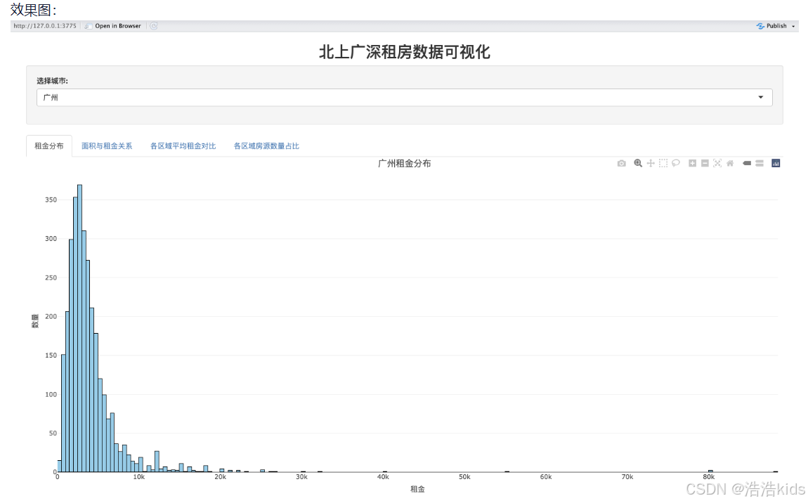

代码
r
# 安装必要的包
install.packages(c("shiny","plotly","dplyr","readr"), repos = "https://mirrors.ustc.edu.cn/CRAN/")
# 导入包,只能一个个导入
library(shiny)
library(plotly)
library(dplyr)
library(readr)
# 查看已导入的包
search()
# 读取数据
data <- read.csv("北上广深租房数据.csv", stringsAsFactors = FALSE) %>%
filter(rent_price_listing > 0, rent_area > 0) %>%
mutate(rent_per_sqm = round(rent_price_listing / rent_area, 2))
# UI 设计
ui <- fluidPage(
titlePanel(h3("北上广深租房数据可视化", align = "center")),
sidebarLayout(
sidebarPanel(
width = 2,
selectInput("city", "选择城市:",
choices = sort(unique(data$city)),
selected = "广州")
),
mainPanel(
tabsetPanel(
tabPanel("租金分布", plotlyOutput("rent_hist", height = "450px")),
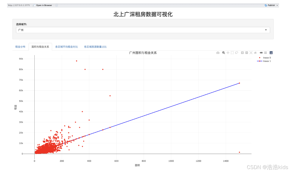
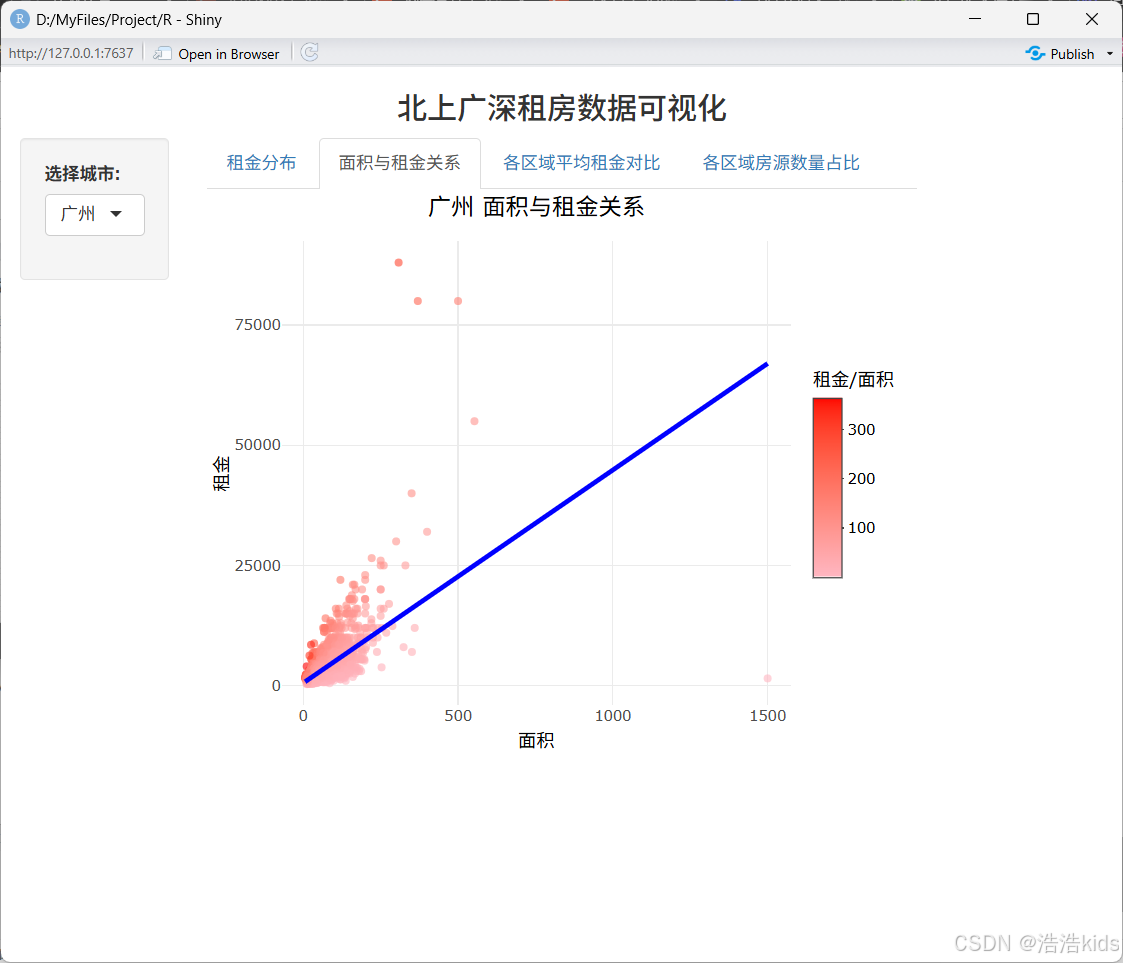
tabPanel("面积与租金关系", plotlyOutput("area_rent_scatter", height = "450px")),
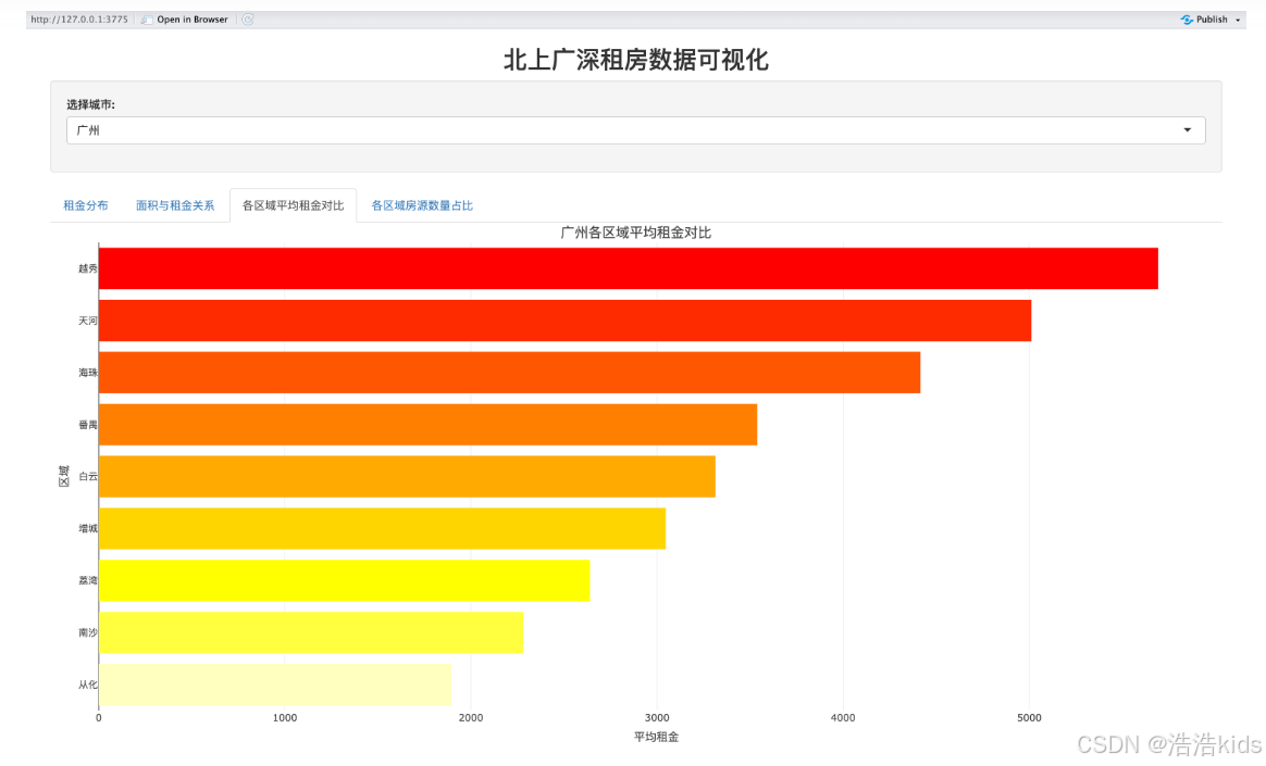
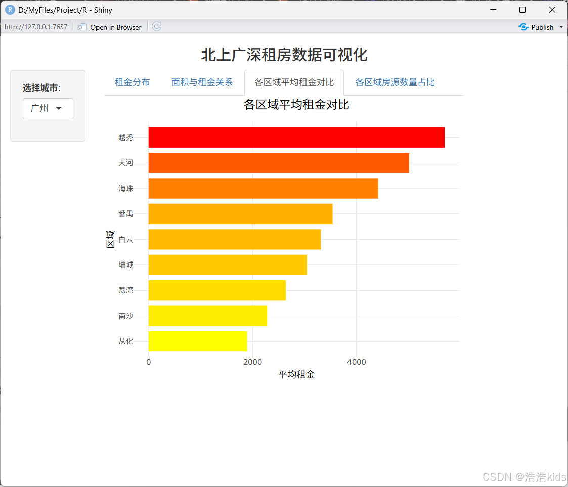
tabPanel("各区域平均租金对比", plotlyOutput("avg_rent_bar", height = "450px")),
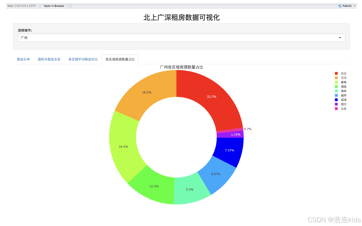
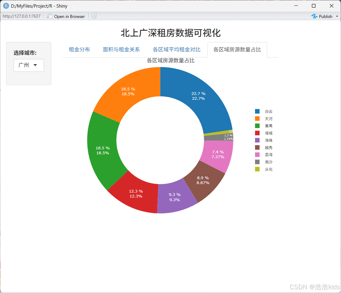
tabPanel("各区域房源数量占比", plotlyOutput("region_pie", height = "450px"))
)
)
)
)
# 服务器逻辑
server <- function(input, output) {
# 过滤数据(根据选中的城市)
filtered_data <- reactive({
data %>% filter(city == input$city)
})
# 租金分布直方图
output$rent_hist <- renderPlotly({
data <- filtered_data()
max_rent <- max(data$rent_price_listing, na.rm = TRUE)
hist_stats <- hist(data$rent_price_listing, bins = 50, plot = FALSE)
max_count <- max(hist_stats$count, na.rm = TRUE)
p <- ggplot(data, aes(x = rent_price_listing)) +
geom_histogram(bins = 50, fill = "#87CEEB", color = "black", alpha = 0.8) +
labs(
title = paste(input$city, "租金分布"),
x = "租金(元/月)",
y = "频数"
) +
scale_x_continuous(
breaks = seq(0, ceiling(max_rent/10000)*10000, 10000),
labels = ~paste0(./1000, "k")
) +
scale_y_continuous(
breaks = seq(0, max_count, 50),
limits = c(0, max_count)
) +
theme_minimal() +
theme(axis.text.y = element_text(size = 5)) # 减小y轴字体大小
ggplotly(p)
})
# 面积与租金关系散点图
output$area_rent_scatter <- renderPlotly({
df <- filtered_data()
p <- ggplot(df, aes(x = rent_area, y = rent_price_listing)) +
geom_point(aes(color = rent_per_sqm), alpha = 0.6, size = 1.2) +
geom_smooth(method = "lm", color = "#0000FF", se = FALSE, linewidth = 1) +
scale_color_gradient(low = "#FFB6C1", high = "#FF0000") +
labs(title = paste(df$city[1], "面积与租金关系"), x = "面积", y = "租金", color = "租金/面积") +
theme_minimal() +
theme(plot.title = element_text(size = 14, hjust = 0.5))
ggplotly(p) %>% config(displayModeBar = FALSE)
})
# 各区域平均租金对比
output$avg_rent_bar <- renderPlotly({
df <- filtered_data() %>%
group_by(dist) %>%
summarise(avg_rent = round(mean(rent_price_listing), 0)) %>%
arrange(desc(avg_rent))
p <- ggplot(df, aes(x = reorder(dist, avg_rent), y = avg_rent)) +
geom_bar(stat = "identity", aes(fill = avg_rent), width = 0.8) +
scale_fill_gradient(low = "#FFFF00", high = "#FF0000") +
coord_flip() +
labs(title = paste(df$city[1], "各区域平均租金对比"), x = "区域", y = "平均租金") +
theme_minimal() +
theme(plot.title = element_text(size = 14, hjust = 0.5), legend.position = "none")
ggplotly(p) %>% config(displayModeBar = FALSE)
})
# 各区域房源数量占比环形图
output$region_pie <- renderPlotly({
df <- filtered_data() %>%
count(dist) %>%
mutate(percentage = round(n / sum(n) * 100, 1)) %>%
arrange(desc(n))
colors <- c("#FF0000", "#FFA500", "#FFFF00", "#008000", "#87CEEB", "#0000FF", "#800080", "#FFC0CB")
p <- plot_ly(
df,
labels = ~dist,
values = ~n,
type = "pie",
hole = 0.6,
colors = colors,
text = ~paste(percentage, "%"),
textposition = "inside",
textfont = list(color = "white", size = 10)
) %>%
layout(
title = list(text = paste(df$city[1], "各区域房源数量占比"), font = list(size = 14), x = 0.5),
legend = list(orientation = "v", x = 1.1, y = 0.5, font = list(size = 10))
)
p %>% config(displayModeBar = FALSE)
})
}
# 运行应用
shinyApp(ui = ui, server = server)效果
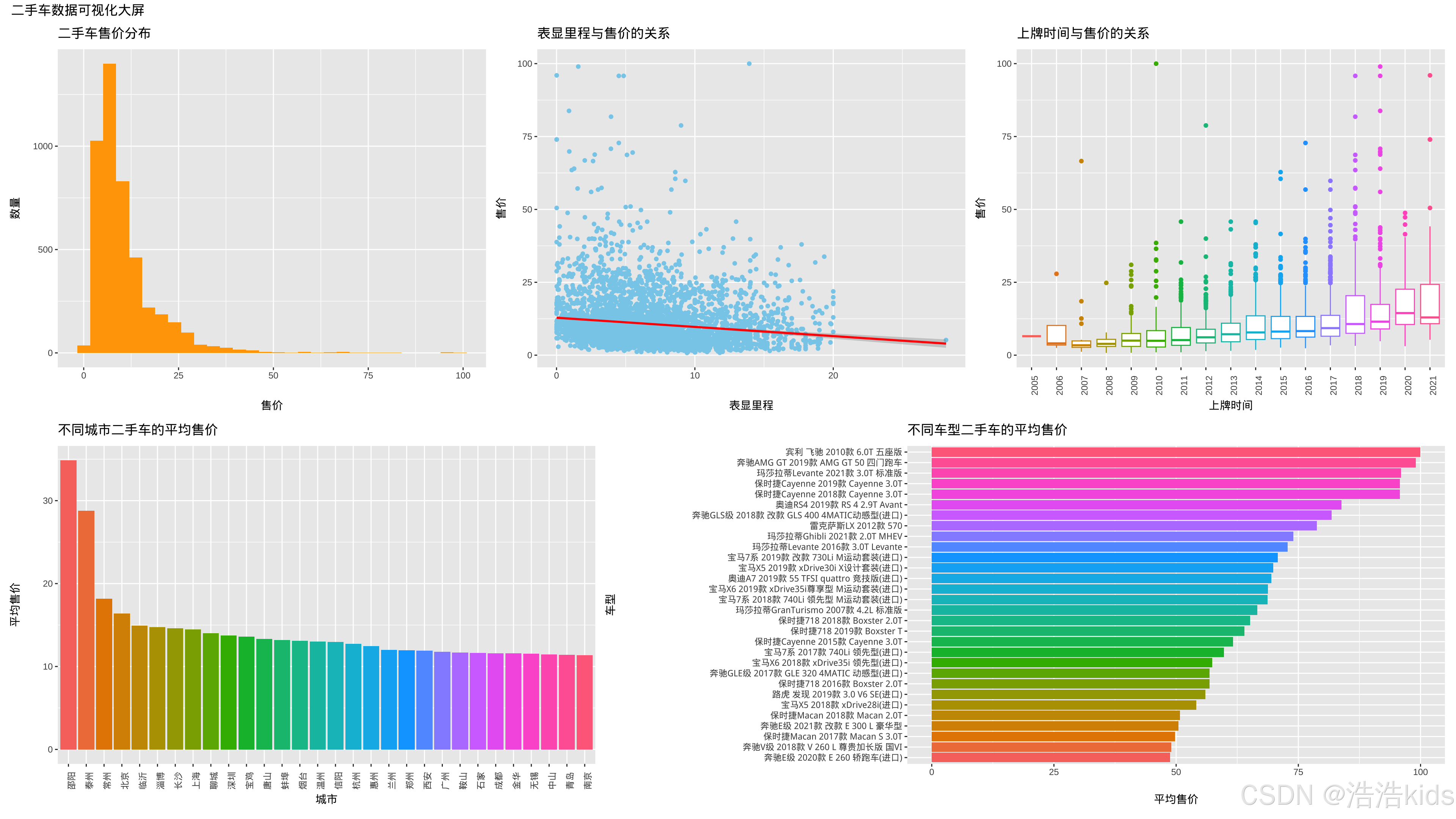
ggplot2绘图

效果图:

代码
r
# 加载必要的包,没有就装,仿照上一题
library(shiny)
library(ggplot2)
library(dplyr)
library(plotly)
library(forcats)
# 读取数据
data <- read.csv("二手车(已处理缺失值、重复值).csv", stringsAsFactors = FALSE) %>%
mutate(上牌时间 = as.integer(上牌时间))
# 定义UI
ui <- fluidPage(
titlePanel(h3("二手车数据可视化大屏", align = "center")),
sidebarLayout(
sidebarPanel(
width = 2,
selectInput("city", "选择城市:",
choices = sort(unique(data$城市)),
multiple = TRUE,
selected = c("北京", "上海", "广州", "深圳")),
selectInput("brand", "选择品牌:",
choices = sort(unique(data$品牌)),
multiple = TRUE,
selected = c("奥迪A4L", "奥迪A6L", "奥迪Q5"))
),
mainPanel(
tabsetPanel(
tabPanel("售价分布", plotlyOutput("price_hist", height = "400px")),
tabPanel("里程与售价", plotlyOutput("mileage_price_scatter", height = "400px")),
tabPanel("上牌时间与售价", plotlyOutput("year_price_box", height = "400px")),
tabPanel("城市平均售价", plotlyOutput("city_price_bar", height = "400px")),
tabPanel("车型平均售价", plotlyOutput("model_price_bar", height = "600px"))
)
)
)
)
# 定义服务器逻辑
server <- function(input, output) {
# 过滤数据
filtered_data <- reactive({
df <- data
if (!is.null(input$city) && length(input$city) > 0) {
df <- df %>% filter(城市 %in% input$city)
}
if (!is.null(input$brand) && length(input$brand) > 0) {
df <- df %>% filter(品牌 %in% input$brand)
}
df
})
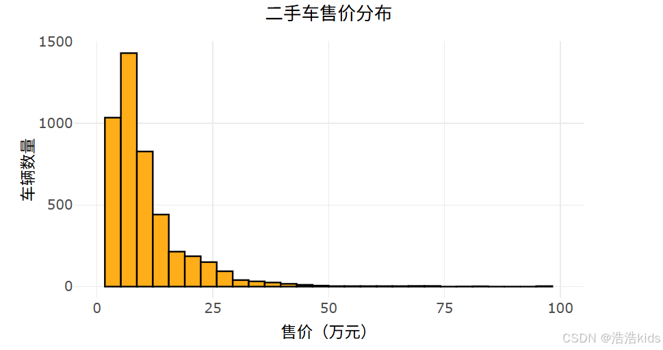
# 1. 二手车售价分布直方图
output$price_hist <- renderPlotly({
df <- filtered_data()
p <- ggplot(df, aes(x = 售价)) +
geom_histogram(fill = "#FFA500", color = "black", bins = 30, alpha = 0.9) +
labs(title = "二手车售价分布", x = "售价(万元)", y = "车辆数量") +
scale_x_continuous(limits = c(0, 100), breaks = seq(0, 100, 25)) +
theme_minimal() +
theme(plot.title = element_text(size = 16, hjust = 0.5),
axis.text = element_text(size = 12),
axis.title = element_text(size = 14))
ggplotly(p) %>% layout(margin = list(t = 50, b = 50))
})
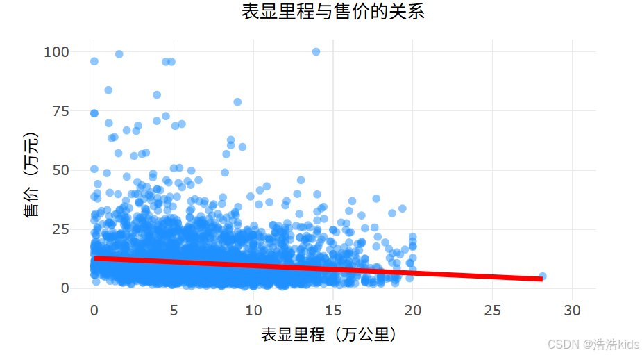
# 2. 表显里程与售价关系散点图
output$mileage_price_scatter <- renderPlotly({
df <- filtered_data()
p <- ggplot(df, aes(x = 表显里程, y = 售价)) +
geom_point(color = "#1E90FF", alpha = 0.5, size = 2) +
geom_smooth(method = "lm", color = "#FF0000", se = FALSE, size = 1.5) +
labs(title = "表显里程与售价的关系", x = "表显里程(万公里)", y = "售价(万元)") +
scale_x_continuous(limits = c(0, 30), breaks = seq(0, 30, 5)) +
scale_y_continuous(limits = c(0, 100), breaks = seq(0, 100, 25)) +
theme_minimal() +
theme(plot.title = element_text(size = 16, hjust = 0.5),
axis.text = element_text(size = 12),
axis.title = element_text(size = 14))
ggplotly(p) %>% layout(margin = list(t = 50, b = 50))
})
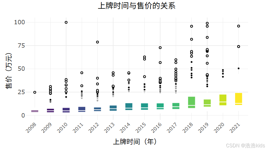
# 3. 上牌时间与售价关系箱线图
output$year_price_box <- renderPlotly({
df <- filtered_data() %>%
filter(上牌时间 >= 2008, 上牌时间 <= 2022) %>%
mutate(上牌时间 = as.factor(上牌时间))
p <- ggplot(df, aes(x = 上牌时间, y = 售价, fill = 上牌时间)) +
geom_boxplot(color = "white", size = 0.5, outlier.shape = 16, outlier.color = "#FF0000") +
scale_fill_viridis_d() +
labs(title = "上牌时间与售价的关系", x = "上牌时间(年)", y = "售价(万元)") +
scale_y_continuous(limits = c(0, 100), breaks = seq(0, 100, 25)) +
theme_minimal() +
theme(plot.title = element_text(size = 16, hjust = 0.5),
axis.text.x = element_text(angle = 45, hjust = 1, size = 10),
axis.text.y = element_text(size = 12),
axis.title = element_text(size = 14),
legend.position = "none")
ggplotly(p) %>% layout(margin = list(t = 50, b = 70))
})
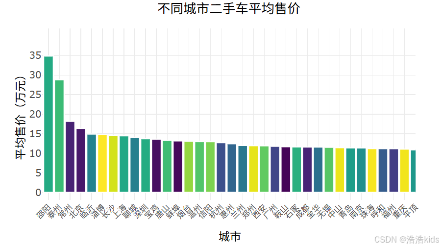
# 4. 不同城市二手车平均售价柱形图
output$city_price_bar <- renderPlotly({
df <- filtered_data()
city_avg <- df %>%
group_by(城市) %>%
summarise(平均售价 = mean(售价, na.rm = TRUE)) %>%
arrange(desc(平均售价))
p <- ggplot(city_avg, aes(x = reorder(城市, -平均售价), y = 平均售价, fill = 城市)) +
geom_col(color = "white", size = 0.2) +
scale_fill_viridis_d() +
labs(title = "不同城市二手车平均售价", x = "城市", y = "平均售价(万元)") +
scale_y_continuous(limits = c(0, max(city_avg$平均售价) + 5), breaks = seq(0, max(city_avg$平均售价) + 5, 5)) +
theme_minimal() +
theme(plot.title = element_text(size = 16, hjust = 0.5),
axis.text.x = element_text(angle = 45, hjust = 1, size = 10),
axis.text.y = element_text(size = 12),
axis.title = element_text(size = 14),
legend.position = "none")
ggplotly(p) %>% layout(margin = list(t = 50, b = 70))
})
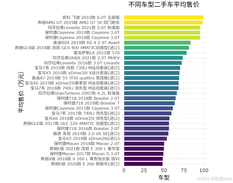
# 5. 不同车型二手车平均售价水平柱形图
output$model_price_bar <- renderPlotly({
df <- filtered_data()
# 检查数据是否为空
if (nrow(df) == 0) {
return(plotly_empty(type = "scatter", mode = "markers") %>%
layout(title = list(text = "没有可用的数据", y = 0.5, x = 0.5, xanchor = "center", yanchor = "center")))
}
# 计算车型平均售价
model_avg <- df %>%
group_by(车型) %>%
summarise(平均售价 = mean(售价, na.rm = TRUE)) %>%
arrange(desc(平均售价))
# 只显示前30个车型,避免图表过于拥挤
if (nrow(model_avg) > 30) {
model_avg <- head(model_avg, 30)
}
p <- ggplot(model_avg, aes(x = reorder(车型, 平均售价), y = 平均售价, fill = 平均售价)) +
geom_col(color = "white", size = 0.2) +
scale_fill_viridis_c() +
labs(title = "不同车型二手车平均售价", x = "平均售价(万元)", y = "车型") +
coord_flip() +
theme_minimal() +
theme(plot.title = element_text(size = 16, hjust = 0.5),
axis.text.y = element_text(size = 10),
axis.text.x = element_text(size = 12),
axis.title = element_text(size = 14),
legend.position = "none")
ggplotly(p, height = 600) %>%
layout(margin = list(t = 50, l = 200))
})
}
# 运行应用
shinyApp(ui = ui, server = server)效果
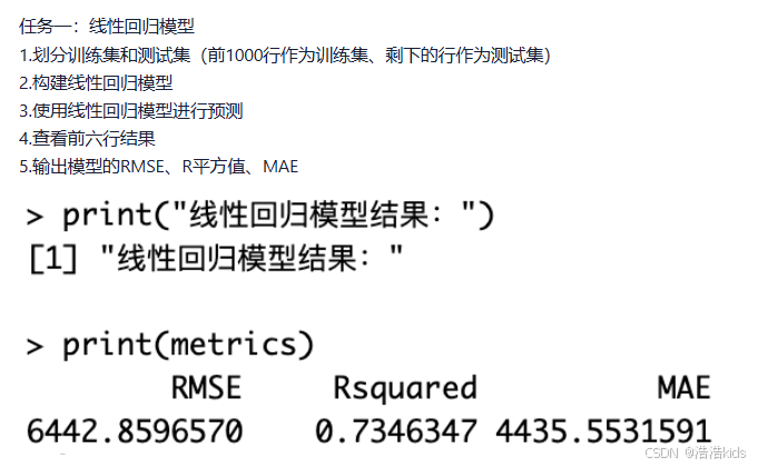
课内实训:医疗保费预测

r
# 1. 读取数据
insurance <- read.csv("insurance.csv")

# 2. 划分训练集和测试集
train_data <- insurance[1:1000, ]
test_data <- insurance[1001:nrow(insurance), ]

# 3. 构建线性回归模型
model <- lm(charges ~ age + sex + bmi + children + smoker + region, data = train_data)

# 4. 使用模型进行预测
predictions <- predict(model, newdata = test_data)

# 5. 查看前六行预测结果
head(predictions)

# 6. 计算模型评估指标
# 实际值
actual <- test_data$charges

# 计算RMSE(均方根误差)
rmse <- sqrt(mean((actual - predictions)^2))

# 计算R平方值
ss_total <- sum((actual - mean(actual))^2)
ss_residual <- sum((actual - predictions)^2)
r_squared <- 1 - (ss_residual / ss_total)

# 计算MAE(平均绝对误差)
mae <- mean(abs(actual - predictions))

# 输出结果
cat("RMSE:", rmse, "\n")
cat("R-squared:", r_squared, "\n")
cat("MAE:", mae, "\n")
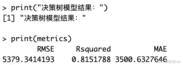
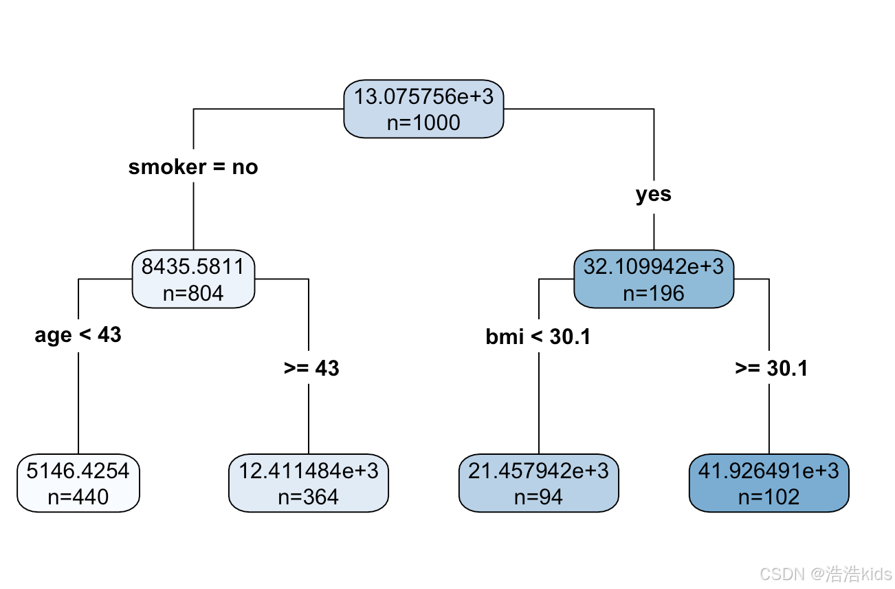
r
# 1. 读取数据,划分训练集和测试集
insurance <- read.csv("insurance.csv")
train_data <- insurance[1:1000, ]
test_data <- insurance[1001:nrow(insurance), ]

# 2. 构建决策树回归模型
# 设置控制参数(可选,用于调整树的复杂度)
tree_control <- rpart.control(minsplit = 10,  # 节点最少样本数
                              minbucket = 5,   # 叶节点最少样本数
                              maxdepth = 10,   # 最大深度
                              cp = 0.01)       # 复杂度参数

# 构建决策树模型
tree_model <- rpart(charges ~ age + sex + bmi + children + smoker + region,
                    data = train_data,
                    method = "anova",
                    control = tree_control)

# 3. 使用决策树模型进行预测
tree_predictions <- predict(tree_model, newdata = test_data)

# 4. 查看前六行预测结果
cat("前六行预测结果:\n")
head(tree_predictions)

# 5. 计算模型评估指标
# 实际值
actual <- test_data$charges

# 计算RMSE(均方根误差)
rmse <- sqrt(mean((actual - tree_predictions)^2))

# 计算R平方值
ss_total <- sum((actual - mean(actual))^2)
ss_residual <- sum((actual - tree_predictions)^2)
r_squared <- 1 - (ss_residual / ss_total)

# 计算MAE(平均绝对误差)
mae <- mean(abs(actual - tree_predictions))

# 输出结果
cat("\n模型评估指标:\n")
cat("RMSE:", round(rmse, 2), "\n")
cat("R-squared:", round(r_squared, 4), "\n")
cat("MAE:", round(mae, 2), "\n")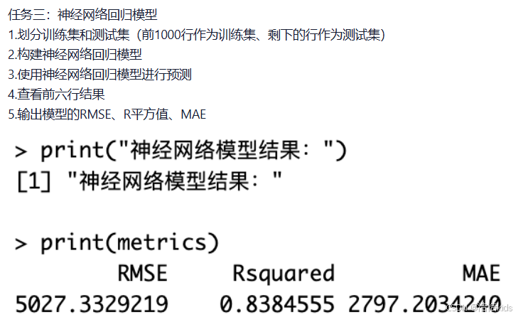
r
# 加载必要的包
library(neuralnet)
library(caret)

# 1. 划分训练集和测试集
# 读取数据
insurance <- read.csv("insurance.csv")

# 数据预处理
# 将分类变量转换为数值变量
insurance$sex <- as.numeric(factor(insurance$sex))
insurance$smoker <- as.numeric(factor(insurance$smoker))
insurance$region <- as.numeric(factor(insurance$region))

# 划分训练集和测试集
train_data <- insurance[1:1000, ]
test_data <- insurance[1001:nrow(insurance), ]

# 2. 构建神经网络回归模型
# 对训练集进行标准化
preprocess_params <- preProcess(train_data[, -7], method = c("center", "scale"))
train_scaled <- predict(preprocess_params, train_data)
test_scaled <- predict(preprocess_params, test_data)

# 设置神经网络公式
nn_formula <- charges ~ age + sex + bmi + children + smoker + region

# 设置神经网络参数
set.seed(123)  # 设置随机种子以保证结果可重现

# 构建神经网络模型
nn_model <- neuralnet(
  nn_formula,
  data = train_scaled,
  hidden = c(5, 3),      # 两个隐藏层,分别有5个和3个神经元
  linear.output = TRUE,  # 回归问题,使用线性输出
  threshold = 0.01,      # 误差函数的偏导数阈值
  stepmax = 1e6          # 最大迭代次数
)

# 3. 使用神经网络模型进行预测
nn_predictions_scaled <- predict(nn_model, test_scaled)

# 将预测结果反标准化
# 获取训练集charges的均值和标准差
charges_mean <- mean(train_data$charges)
charges_sd <- sd(train_data$charges)

# 反标准化预测结果
nn_predictions <- nn_predictions_scaled * charges_sd + charges_mean

# 4. 查看前六行预测结果
cat("前六行预测结果:\n")
head(nn_predictions)

# 5. 计算模型评估指标
# 实际值
actual <- test_data$charges

# 计算RMSE(均方根误差)
rmse <- sqrt(mean((actual - nn_predictions)^2))

# 计算R平方值
ss_total <- sum((actual - mean(actual))^2)
ss_residual <- sum((actual - nn_predictions)^2)
r_squared <- 1 - (ss_residual / ss_total)

# 计算MAE(平均绝对误差)
mae <- mean(abs(actual - nn_predictions))

# 输出结果
cat("\n神经网络模型评估指标:\n")
cat("RMSE:", round(rmse, 2), "\n")
cat("R-squared:", round(r_squared, 4), "\n")
cat("MAE:", round(mae, 2), "\n")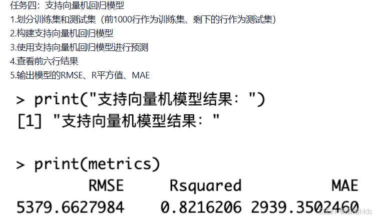
r
# 加载必要的包
library(e1071)
library(caret)

# 1. 划分训练集和测试集
# 读取数据
insurance <- read.csv("insurance.csv")

# 数据预处理
# 将分类变量转换为数值变量
insurance$sex <- as.numeric(factor(insurance$sex))
insurance$smoker <- as.numeric(factor(insurance$smoker))
insurance$region <- as.numeric(factor(insurance$region))

# 划分训练集和测试集
train_data <- insurance[1:1000, ]
test_data <- insurance[1001:nrow(insurance), ]

# 数据标准化(SVM对数据尺度敏感)
# 对训练集进行标准化
preprocess_params <- preProcess(train_data[, -7], method = c("center", "scale"))
train_scaled <- predict(preprocess_params, train_data)
test_scaled <- predict(preprocess_params, test_data)

# 2. 构建支持向量机回归模型
# 设置SVM参数
set.seed(123)  # 设置随机种子以保证结果可重现

# 构建SVM回归模型
svm_model <- svm(charges ~ age + sex + bmi + children + smoker + region,
                 data = train_scaled,
                 type = "eps-regression",  # 回归类型
                 kernel = "radial",         # 径向基核函数
                 cost = 1,                 # 惩罚参数
                 gamma = 0.1,              # 核函数参数
                 epsilon = 0.1)            # 不敏感损失函数参数

# 3. 使用SVM模型进行预测
svm_predictions_scaled <- predict(svm_model, test_scaled)

# 将预测结果反标准化
# 获取训练集charges的均值和标准差
charges_mean <- mean(train_data$charges)
charges_sd <- sd(train_data$charges)

# 反标准化预测结果
svm_predictions <- svm_predictions_scaled * charges_sd + charges_mean

# 4. 查看前六行预测结果
cat("前六行预测结果:\n")
head(svm_predictions)

# 5. 计算模型评估指标
# 实际值
actual <- test_data$charges

# 计算RMSE(均方根误差)
rmse <- sqrt(mean((actual - svm_predictions)^2))

# 计算R平方值
ss_total <- sum((actual - mean(actual))^2)
ss_residual <- sum((actual - svm_predictions)^2)
r_squared <- 1 - (ss_residual / ss_total)

# 计算MAE(平均绝对误差)
mae <- mean(abs(actual - svm_predictions))

# 输出结果
cat("\n支持向量机回归模型评估指标:\n")
cat("RMSE:", round(rmse, 2), "\n")
cat("R-squared:", round(r_squared, 4), "\n")
cat("MAE:", round(mae, 2), "\n")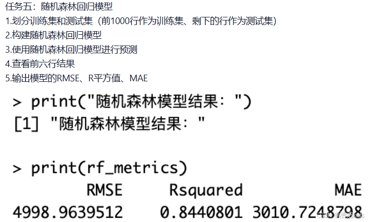
r
# 加载必要的包
library(randomForest)
library(caret)

# 1. 划分训练集和测试集
# 读取数据
insurance <- read.csv("insurance.csv")

# 数据预处理
# 将分类变量转换为因子
insurance$sex <- as.factor(insurance$sex)
insurance$smoker <- as.factor(insurance$smoker)
insurance$region <- as.factor(insurance$region)

# 划分训练集和测试集
train_data <- insurance[1:1000, ]
test_data <- insurance[1001:nrow(insurance), ]

# 2. 构建随机森林回归模型
set.seed(123)  # 设置随机种子以保证结果可重现

# 构建随机森林模型
rf_model <- randomForest(charges ~ age + sex + bmi + children + smoker + region,
                         data = train_data,
                         ntree = 500,        # 树的数量
                         mtry = 3,           # 每棵树使用的特征数
                         importance = TRUE,  # 计算特征重要性
                         na.action = na.omit)

# 3. 使用随机森林模型进行预测
rf_predictions <- predict(rf_model, newdata = test_data)

# 4. 查看前六行预测结果
cat("前六行预测结果:\n")
head(rf_predictions)

# 5. 计算模型评估指标
# 实际值
actual <- test_data$charges

# 计算RMSE(均方根误差)
rmse <- sqrt(mean((actual - rf_predictions)^2))

# 计算R平方值
ss_total <- sum((actual - mean(actual))^2)
ss_residual <- sum((actual - rf_predictions)^2)
r_squared <- 1 - (ss_residual / ss_total)

# 计算MAE(平均绝对误差)
mae <- mean(abs(actual - rf_predictions))

# 输出结果
cat("\n随机森林回归模型评估指标:\n")
cat("RMSE:", round(rmse, 2), "\n")
cat("R-squared:", round(r_squared, 4), "\n")
cat("MAE:", round(mae, 2), "\n")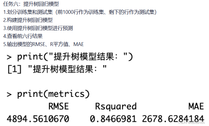
r
# 加载必要的包
library(gbm)
library(caret)

# 1. 划分训练集和测试集
# 读取数据
insurance <- read.csv("insurance.csv")

# 数据预处理
# 将分类变量转换为数值变量
insurance$sex <- as.numeric(factor(insurance$sex))
insurance$smoker <- as.numeric(factor(insurance$smoker))
insurance$region <- as.numeric(factor(insurance$region))

# 划分训练集和测试集
train_data <- insurance[1:1000, ]
test_data <- insurance[1001:nrow(insurance), ]

# 2. 构建提升树回归模型
set.seed(123)  # 设置随机种子以保证结果可重现

# 构建GBM模型
gbm_model <- gbm(charges ~ age + sex + bmi + children + smoker + region,
                 data = train_data,
                 distribution = "gaussian",      # 高斯分布(回归问题)
                 n.trees = 1000,                 # 树的数量
                 interaction.depth = 4,          # 树的深度
                 shrinkage = 0.01,              # 学习率
                 cv.folds = 5,                   # 交叉验证折数
                 n.minobsinnode = 10,           # 叶节点最小观测数
                 verbose = FALSE)               # 不显示详细过程

# 3. 使用提升树模型进行预测
gbm_predictions <- predict(gbm_model, newdata = test_data, n.trees = 1000)

# 4. 查看前六行预测结果
cat("前六行预测结果:\n")
head(gbm_predictions)

# 5. 计算模型评估指标
# 实际值
actual <- test_data$charges

# 计算RMSE(均方根误差)
rmse <- sqrt(mean((actual - gbm_predictions)^2))

# 计算R平方值
ss_total <- sum((actual - mean(actual))^2)
ss_residual <- sum((actual - gbm_predictions)^2)
r_squared <- 1 - (ss_residual / ss_total)

# 计算MAE(平均绝对误差)
mae <- mean(abs(actual - gbm_predictions))

# 输出结果
cat("\n提升树回归模型评估指标:\n")
cat("RMSE:", round(rmse, 2), "\n")
cat("R-squared:", round(r_squared, 4), "\n")
cat("MAE:", round(mae, 2), "\n")
餐饮企业客户价值分析

r
library(dendextend)
library(xlsx)
# 1. 读取数据,移除 Id 列
# 读取数据
data <- read.xlsx("餐饮企业客户价值分析.xls", sheetIndex = 1)
# 查看数据结构
cat("数据维度:", dim(data), "\n")
cat("前几行数据:\n")
print(head(data))
# 移除 Id 列
data <- data[, -1]
# 2. 数据标准化
scaled_data <- scale(data)
# 3. 计算距离矩阵
dist_matrix <- dist(scaled_data, method = "euclidean")
# 4. 进行层次聚类
hc <- hclust(dist_matrix, method = "ward.D2")
# 5. 使用dendextend可视化层次聚类结果
# 将层次聚类结果转换为树状图对象
dend <- as.dendrogram(hc)
# 设置颜色和样式
dend <- dend %>%
set("branches_k_color", k = 3) %>% # 设置3个主要分支的颜色
set("branches_lwd", 1.2) %>% # 设置分支线宽
set("labels_col", "darkblue") %>% # 设置标签颜色
set("labels_cex", 0.3) %>% # 设置标签大小
set("leaves_pch", 19) %>% # 设置叶子标记形状
set("leaves_cex", 0.5) # 设置叶子标记大小
# 设置图形参数
par(mar = c(5, 4, 4, 8)) # 增加右边距用于图例
# 绘制改进的树状图
plot(dend,
main = "餐饮企业客户价值层次聚类分析",
ylab = "距离高度",
xlab = "客户样本",
leaflab = "none", # 不显示叶子标签避免重叠
axes = TRUE)
# 添加聚类划分(分为3类)
rect.dendrogram(dend, k = 3, border = 2:4, lty = 2, lwd = 2)
# 添加图例
legend("topright",
legend = c("聚类1: 低价值客户", "聚类2: 中等价值客户", "聚类3: 高价值客户"),
fill = 2:4,
bty = "n",
cex = 0.8,
xpd = TRUE, # 允许在图外绘制
inset = c(-0.25, 0)) # 调整图例位置
# 添加网格线以便更好地读取高度
grid(nx = NA, ny = NULL, lty = 2, col = "gray")
# 聚类结果分析
# 将数据分为3类
clusters <- cutree(hc, k = 3)
# 查看每类的样本数量
cluster_counts <- table(clusters)
cat("\n聚类结果统计:\n")
print(cluster_counts)
# 将聚类结果添加到原始数据
data_with_clusters <- cbind(data, Cluster = clusters)
# 查看各聚类中心的统计信息
cluster_stats <- aggregate(data, by = list(Cluster = clusters), FUN = mean)
cat("\n各聚类中心统计信息:\n")
print(cluster_stats)
# 计算各聚类的标准差
cluster_sd <- aggregate(data, by = list(Cluster = clusters), FUN = sd)
cat("\n各聚类标准差:\n")
print(cluster_sd)
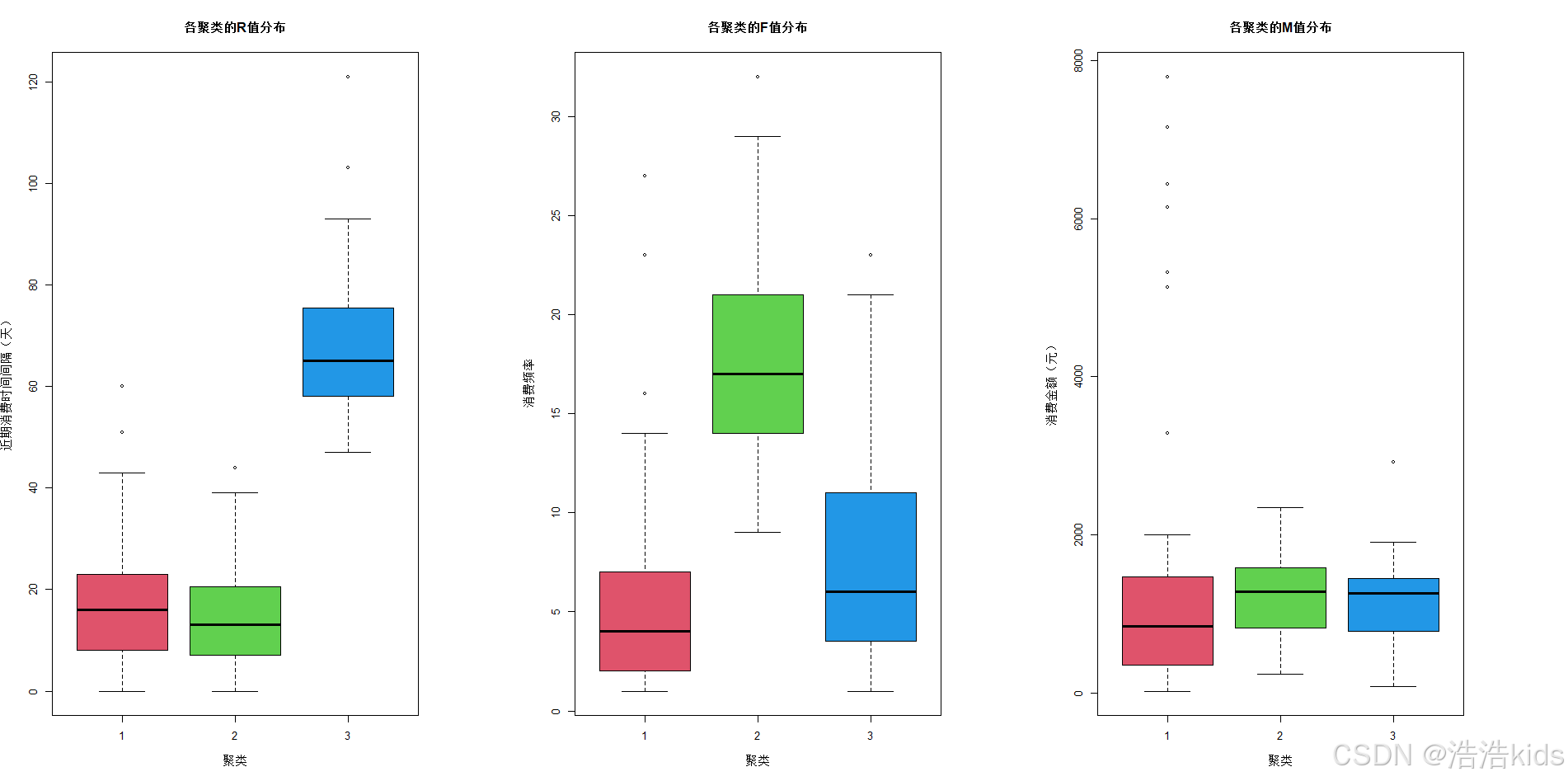
# 可视化聚类特征
# 使用箱线图展示各聚类在R、F、M变量上的分布
par(mfrow = c(1, 3)) # 设置1行3列的图形布局
boxplot(R ~ Cluster, data = data_with_clusters,
main = "各聚类的R值分布",
xlab = "聚类", ylab = "近期消费时间间隔(天)",
col = 2:4)
boxplot(F ~ Cluster, data = data_with_clusters,
main = "各聚类的F值分布",
xlab = "聚类", ylab = "消费频率",
col = 2:4)
boxplot(M ~ Cluster, data = data_with_clusters,
main = "各聚类的M值分布",
xlab = "聚类", ylab = "消费金额(元)",
col = 2:4)
# 重置图形参数
par(mfrow = c(1, 1))
# 8. 保存聚类结果
# 将带有聚类结果的数据保存为CSV文件
write.csv(data_with_clusters, "客户价值聚类结果.csv", row.names = FALSE)
cat("\n聚类结果已保存到 '客户价值聚类结果.csv'\n")
# 输出聚类分析总结
cat("\n=== 聚类分析总结 ===\n")
cat("总客户数:", nrow(data), "\n")
cat("聚类数量: 3\n")
cat("聚类方法: Ward层次聚类\n")
cat("距离度量: 欧氏距离\n")
cat("数据标准化: 是\n")
for(i in 1:3) {
cat("\n聚类", i, "特征:\n")
cat(" 客户数量:", cluster_counts[i], "\n")
cat(" 平均R值:", round(cluster_stats$R[i], 2), "\n")
cat(" 平均F值:", round(cluster_stats$F[i], 2), "\n")
cat(" 平均M值:", round(cluster_stats$M[i], 2), "\n")
}

r
# 加载必要的包
library(xlsx)
library(ggplot2)
library(dplyr)
library(RColorBrewer)

# 1. 读取数据、移除 Id 列
data <- read.xlsx("餐饮企业客户价值分析.xls", sheetIndex = 1)
data <- data[, -1]

# 2. 数据标准化
scaled_data <- scale(data)

# 3. 进行 K-Means 聚类
set.seed(123)  # 设置随机种子保证结果可重现
kmeans_result <- kmeans(scaled_data, centers = 3, nstart = 25)

# 4. 查看聚类中心
print("聚类中心:")
print(kmeans_result$centers)

# 5. 将聚类标签添加到原始数据中
data$Cluster <- kmeans_result$cluster

# 6. 替换聚类标签为对应的客户价值类别
# 根据聚类中心分析客户价值类型
cluster_centers <- kmeans_result$centers
cluster_labels <- c("低价值客户", "中等价值客户", "高价值客户")

# 根据R值(近期消费时间间隔)和M值(消费金额)确定客户价值
# R值越小越好(近期有消费),M值越大越好
r_ranks <- order(cluster_centers[, "R"])  # R值排序,值越小排名越高
m_ranks <- order(-cluster_centers[, "M"])  # M值排序,值越大排名越高

# 综合排名确定客户价值类别
combined_ranks <- (r_ranks + m_ranks) / 2
value_order <- order(combined_ranks)

# 创建价值类别映射
value_mapping <- data.frame(
  Cluster = 1:3,
  ValueType = cluster_labels[value_order]
)

# 将数值标签替换为价值类别
data$ValueType <- factor(data$Cluster,
                         levels = value_mapping$Cluster,
                         labels = value_mapping$ValueType)

# 7. 保存结果到 csv 文件
write.csv(data, "KMeans聚类结果.csv", row.names = FALSE)

# 8. 统计每个聚类类别的数量
cluster_counts <- table(data$ValueType)
print("各价值类别客户数量:")
print(cluster_counts)

# 9. 绘制不同价值客户占比环形图
value_summary <- data %>%
  group_by(ValueType) %>%
  summarise(Count = n()) %>%
  mutate(Percentage = Count/sum(Count)*100,
         ymax = cumsum(Percentage),
         ymin = c(0, head(ymax, n = -1)),
         label = paste0(ValueType, "\n", round(Percentage, 1), "%"))

# 创建环形图
ggplot(value_summary, aes(ymax = ymax, ymin = ymin,
                          xmax = 4, xmin = 3, fill = ValueType)) +
  geom_rect(color = "white", size = 0.5) +
  geom_text(aes(x = 3.5, y = (ymin + ymax)/2, label = label),
            size = 3, color = "white", lineheight = 0.8) +
  scale_fill_manual(values = c("#E41A1C", "#377EB8", "#4DAF4A")) +
  coord_polar(theta = "y") +
  xlim(c(1.5, 4)) +
  theme_void() +
  theme(
    legend.position = "none",
    plot.title = element_text(
      size = 16,
      face = "bold",
      hjust = 0.5,
      vjust = 1,
      margin = margin(b = 10)
    )
  ) +
  labs(
    title = "客户价值分布环形图",
    subtitle = paste("总客户数:", nrow(data))
  ) +
  annotate("rect", xmin = 1.5, xmax = 2.5, ymin = 0, ymax = 100,
           fill = "white", color = NA)

# 保存环形图
ggsave("客户价值分布环形图.png", width = 10, height = 8, dpi = 300, bg = "white")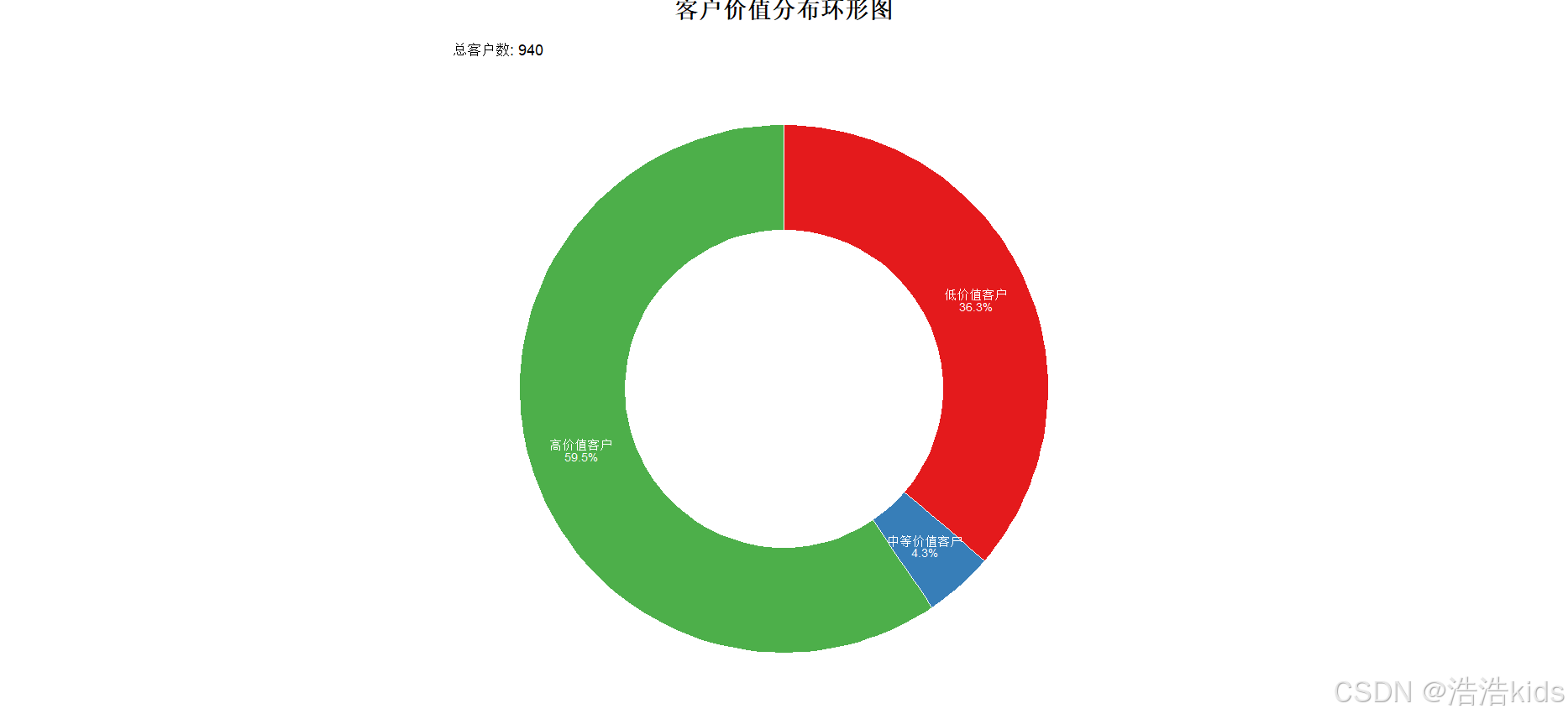
航空公司客户价值分析

r
# 加载必要的包
library(xlsx)
library(ggplot2)
library(dplyr)
library(RColorBrewer)

# 1. 读取数据、移除 Id 列
data <- read.xlsx("air_features.xlsx", sheetIndex = 1)
data <- data[, -1]

# 2. 数据标准化
scaled_data <- scale(data)

# 3. 进行 K-Means 聚类
set.seed(123)  # 设置随机种子保证结果可重现
kmeans_result <- kmeans(scaled_data, centers = 3, nstart = 25)

# 4. 查看聚类中心
print("聚类中心:")
print(kmeans_result$centers)

# 5. 将聚类标签添加到原始数据中
data$Cluster <- kmeans_result$cluster

# 6. 替换聚类标签为对应的客户价值类别
# 根据聚类中心分析客户价值类型
cluster_centers <- kmeans_result$centers
cluster_labels <- c("低价值客户", "中等价值客户", "高价值客户")

# 根据R值(近期消费时间间隔)和M值(消费金额)确定客户价值
# R值越小越好(近期有消费),M值越大越好
r_ranks <- order(cluster_centers[, "R"])  # R值排序,值越小排名越高
m_ranks <- order(-cluster_centers[, "M"])  # M值排序,值越大排名越高

# 综合排名确定客户价值类别
combined_ranks <- (r_ranks + m_ranks) / 2
value_order <- order(combined_ranks)

# 创建价值类别映射
value_mapping <- data.frame(
  Cluster = 1:3,
  ValueType = cluster_labels[value_order]
)

# 将数值标签替换为价值类别
data$ValueType <- factor(data$Cluster,
                         levels = value_mapping$Cluster,
                         labels = value_mapping$ValueType)

# 7. 保存结果到 csv 文件
write.csv(data, "KMeans聚类结果.csv", row.names = FALSE)

# 8. 统计每个聚类类别的数量
cluster_counts <- table(data$ValueType)
print("各价值类别客户数量:")
print(cluster_counts)

# 9. 绘制不同价值客户占比环形图
value_summary <- data %>%
  group_by(ValueType) %>%
  summarise(Count = n()) %>%
  mutate(Percentage = Count/sum(Count)*100,
         ymax = cumsum(Percentage),
         ymin = c(0, head(ymax, n = -1)),
         label = paste0(ValueType, "\n", round(Percentage, 1), "%"))

# 创建环形图
ggplot(value_summary, aes(ymax = ymax, ymin = ymin,
                          xmax = 4, xmin = 3, fill = ValueType)) +
  geom_rect(color = "white", size = 0.5) +
  geom_text(aes(x = 3.5, y = (ymin + ymax)/2, label = label),
            size = 3, color = "white", lineheight = 0.8) +
  scale_fill_manual(values = c("#E41A1C", "#377EB8", "#4DAF4A")) +
  coord_polar(theta = "y") +
  xlim(c(1.5, 4)) +
  theme_void() +
  theme(
    legend.position = "none",
    plot.title = element_text(
      size = 16,
      face = "bold",
      hjust = 0.5,
      vjust = 1,
      margin = margin(b = 10)
    )
  ) +
  labs(
    title = "客户价值分布环形图",
    subtitle = paste("总客户数:", nrow(data))
  ) +
  annotate("rect", xmin = 1.5, xmax = 2.5, ymin = 0, ymax = 100,
           fill = "white", color = NA)

# 保存环形图
ggsave("客户价值分布环形图.png", width = 10, height = 8, dpi = 300, bg = "white")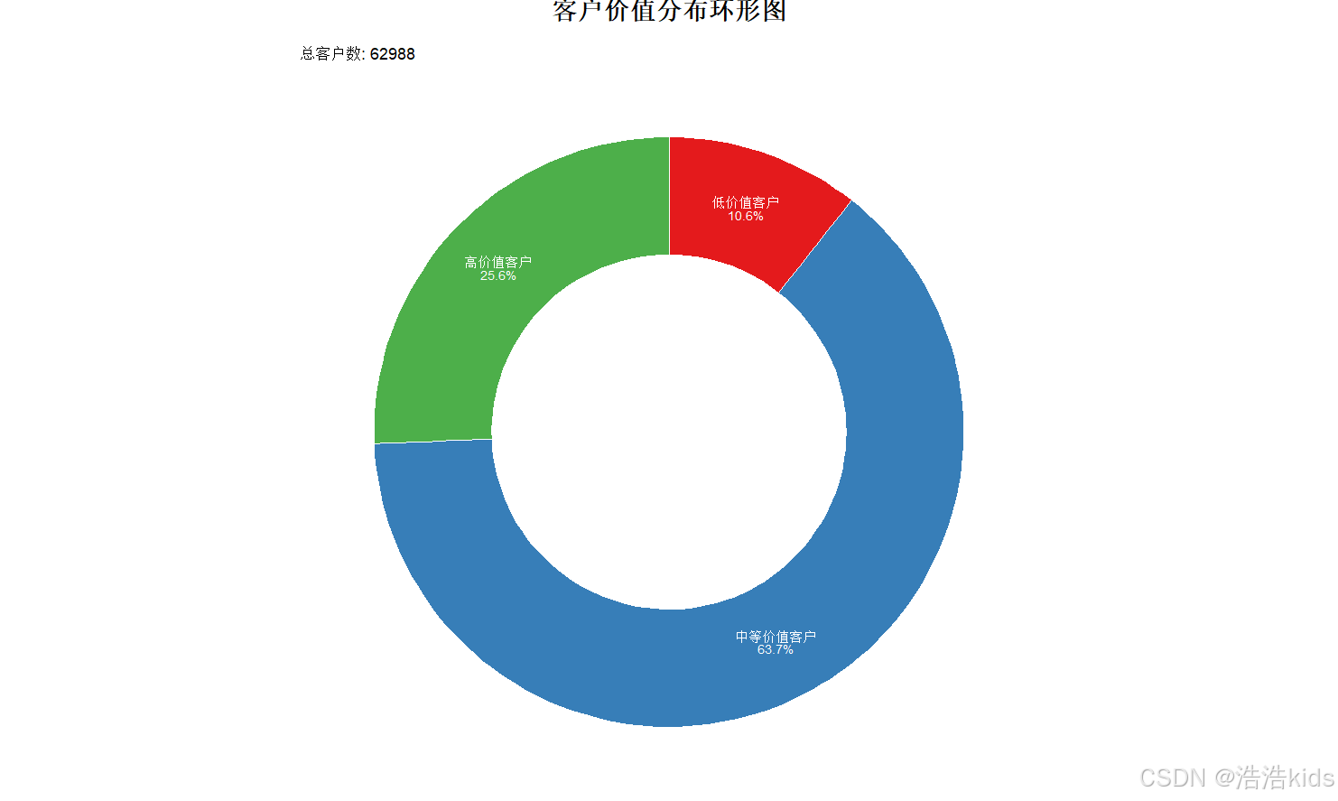
课内实训:通信企业客户流失预测


r
install.packages("tidyverse")
install.packages("caret")
install.packages("rpart")
chooseCRANmirror()
install.packages("rpart.plot")
install.packages("nnet")
install.packages("e1071")
install.packages("randomForest")
install.packages("gbm")
# 加载包
library(tidyverse) # 数据处理与可视化
library(caret) # 数据划分、模型评估
library(rpart) # 决策树模型
library(rpart.plot) # 决策树可视化
library(nnet) # 神经网络模型
library(e1071) # 支持向量机模型
library(randomForest) # 随机森林模型
library(gbm) # 梯度提升机模型
# 设置随机种子(保证结果可重复)
set.seed(123)
# 读取数据
data <- read.csv("D://myTemp//homework//R//作业数据源//communication.csv", stringsAsFactors = FALSE)
# 查看数据基本信息
cat("数据维度:", dim(data), "\n") # 查看数据行数和列数
cat("\n数据前5行:\n")
print(head(data, 5))
cat("\n数据类型:\n")
print(str(data))
cat("\n缺失值检查:\n")
print(colSums(is.na(data))) # 检查各列缺失值(本次数据无缺失)
#任务一:逻辑回归模型
#分离特征和目标变量
# 定义特征变量和目标变量(type为目标变量:0=未流失,1=已流失)
features <- data[, c("age", "educational_level", "months", "electronic_payment")]
target <- factor(data$type, levels = c(0, 1), labels = c("未流失", "已流失"))
#划分训练集和测试集
# 划分训练集(70%)和测试集(30%)
train_index <- createDataPartition(target, p = 0.7, list = FALSE)
train_features <- features[train_index, ]
test_features <- features[-train_index, ]
train_target <- target[train_index]
test_target <- target[-train_index]
#构建逻辑回归模型
lr_model <- glm(
formula = train_target ~ .,
data = data.frame(train_features, train_target),
family = binomial(link = "logit")
)
# 查看模型摘要
cat("逻辑回归模型摘要:\n")
print(summary(lr_model))
#进行预测
# 在测试集上预测(输出概率,再转换为类别)
lr_prob <- predict(lr_model, newdata = test_features, type = "response")
lr_pred <- ifelse(lr_prob > 0.5, "已流失", "未流失")
lr_pred <- factor(lr_pred, levels = c("未流失", "已流失")) # 与目标变量格式一致
#查看前六行结果
cat("\n逻辑回归预测结果(前6行):\n")
result_lr <- data.frame(
测试集索引 = 1:6,
实际标签 = test_target[1:6],
预测标签 = lr_pred[1:6],
流失概率 = round(lr_prob[1:6], 4)
)
print(result_lr)
#输出预测结果、混淆矩阵、准确率
# 混淆矩阵(行=实际类别,列=预测类别)
cat("\n逻辑回归混淆矩阵:\n")
lr_cm <- confusionMatrix(lr_pred, test_target)
print(lr_cm$table)
# 模型准确率及其他评估指标
cat("\n逻辑回归模型评估:\n")
cat("准确率:", round(lr_cm$overall["Accuracy"], 4), "\n")
cat("精确率(已流失):", round(lr_cm$byClass["Precision2"], 4), "\n")
cat("召回率(已流失):", round(lr_cm$byClass["Recall2"], 4), "\n")
cat("F1分数(已流失):", round(lr_cm$byClass["F12"], 4), "\n")
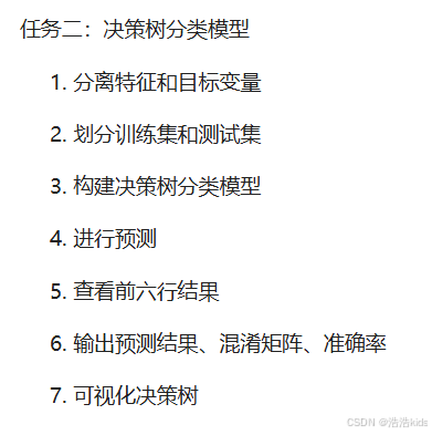
#任务二:决策树分类模型
#分离特征和目标变量
#任务一已做完
#划分训练集和测试集
#任务一已做完
#构建决策树分类模型(限制树深度为3,避免过拟合)
dt_model <- rpart(
formula = train_target ~ .,
data = data.frame(train_features, train_target),
control = rpart.control(maxdepth = 3, minsplit = 10)
)
#进行预测
dt_pred <- predict(dt_model, newdata = test_features, type = "class")
#查看前六行结果
cat("\n决策树预测结果(前6行):\n")
result_dt <- data.frame(
测试集索引 = 1:6,
实际标签 = test_target[1:6],
预测标签 = dt_pred[1:6]
)
print(result_dt)
#输出预测结果、混淆矩阵、准确率
# 混淆矩阵
cat("\n决策树混淆矩阵:\n")
dt_cm <- confusionMatrix(dt_pred, test_target)
print(dt_cm$table)
# 模型评估
cat("\n决策树模型评估:\n")
cat("准确率:", round(dt_cm$overall["Accuracy"], 4), "\n")
cat("精确率(已流失):", round(dt_cm$byClass["Precision2"], 4), "\n")
cat("召回率(已流失):", round(dt_cm$byClass["Recall2"], 4), "\n")
cat("F1分数(已流失):", round(dt_cm$byClass["F12"], 4), "\n")
#可视化决策树
# 绘制决策树(保存为图片)
png("决策树可视化.png", width = 800, height = 600)
rpart.plot(
dt_model,
main = "通信企业客户流失预测决策树",
extra = 101, # 显示节点样本数和类别比例
under = TRUE, # 在节点下方显示类别
faclen = 0, # 不缩写变量名
cex = 0.8 # 字体大小
)
dev.off()
cat("\n决策树已保存为'决策树可视化.png'\n")
#任务三:神经网络分类模型
#分离特征和目标变量
#任务一已做完
#划分训练集和测试集
#任务一已做完
#构建神经网络分类模型
# 特征标准化(神经网络对特征尺度敏感,需标准化)
preprocess <- preProcess(train_features, method = c("center", "scale"))
train_features_scaled <- predict(preprocess, train_features)
test_features_scaled <- predict(preprocess, test_features)
# 构建神经网络模型(size=5为隐藏层节点数,maxit=1000为最大迭代次数)
nn_model <- nnet(
formula = train_target ~ .,
data = data.frame(train_features_scaled, train_target),
size = 5,
maxit = 1000,
decay = 0.01, # 正则化参数,避免过拟合
trace = FALSE # 不显示迭代过程
)
#进行预测
nn_pred <- predict(nn_model, newdata = test_features_scaled, type = "class")
nn_pred <- factor(nn_pred, levels = c("未流失", "已流失"))
#查看前六行结果
cat("\n神经网络预测结果(前6行):\n")
result_nn <- data.frame(
测试集索引 = 1:6,
实际标签 = test_target[1:6],
预测标签 = nn_pred[1:6]
)
print(result_nn)
#输出预测结果、混淆矩阵、准确率
# 混淆矩阵
cat("\n神经网络混淆矩阵:\n")
nn_cm <- confusionMatrix(nn_pred, test_target)
print(nn_cm$table)
# 模型评估
cat("\n神经网络模型评估:\n")
cat("准确率:", round(nn_cm$overall["Accuracy"], 4), "\n")
cat("精确率(已流失):", round(nn_cm$byClass["Precision2"], 4), "\n")
cat("召回率(已流失):", round(nn_cm$byClass["Recall2"], 4), "\n")
cat("F1分数(已流失):", round(nn_cm$byClass["F12"], 4), "\n")
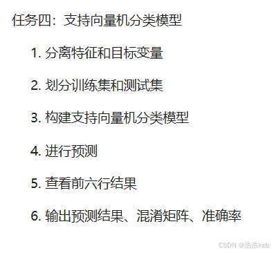
#任务四:支持向量机分类模型
#分离特征和目标变量
#任务一已做完
#划分训练集和测试集
#任务一已做完
#构建支持向量机分类模型
svm_model <- svm(
formula = train_target ~ .,
data = data.frame(train_features_scaled, train_target),
kernel = "radial",
cost = 1, # 惩罚参数
gamma = 0.25, # 核函数参数
probability = TRUE # 允许输出概率
)
#进行预测
svm_pred <- predict(svm_model, newdata = test_features_scaled, type = "class")
#查看前六行结果
cat("\n支持向量机预测结果(前6行):\n")
result_svm <- data.frame(
测试集索引 = 1:6,
实际标签 = test_target[1:6],
预测标签 = svm_pred[1:6]
)
print(result_svm)
#输出预测结果、混淆矩阵、准确率
# 混淆矩阵
cat("\n支持向量机混淆矩阵:\n")
svm_cm <- confusionMatrix(svm_pred, test_target)
print(svm_cm$table)
# 模型评估
cat("\n支持向量机模型评估:\n")
cat("准确率:", round(svm_cm$overall["Accuracy"], 4), "\n")
cat("精确率(已流失):", round(svm_cm$byClass["Precision2"], 4), "\n")
cat("召回率(已流失):", round(svm_cm$byClass["Recall2"], 4), "\n")
cat("F1分数(已流失):", round(svm_cm$byClass["F12"], 4), "\n")
#任务五:随机森林分类模型
#分离特征和目标变量
#任务一已做完
#划分训练集和测试集
#任务一已做完
#构建随机森林分类模型(ntree=500为决策树数量,mtry=2为每棵树使用的特征数)
rf_model <- randomForest(
formula = train_target ~ .,
data = data.frame(train_features, train_target),
ntree = 500,
mtry = 2,
importance = TRUE, # 计算特征重要性
proximity = FALSE
)
# 查看特征重要性
cat("\n随机森林特征重要性:\n")
print(importance(rf_model))
par(mar = c(5,4,4,2)+0.1) # 调整边距,数值可根据需要微调
varImpPlot(rf_model, main = "特征重要性排序")
#进行预测
rf_pred <- predict(rf_model, newdata = test_features, type = "class")
#查看前六行结果
cat("\n随机森林预测结果(前6行):\n")
result_rf <- data.frame(
测试集索引 = 1:6,
实际标签 = test_target[1:6],
预测标签 = rf_pred[1:6]
)
print(result_rf)
#输出预测结果、混淆矩阵、准确率
# 混淆矩阵
cat("\n随机森林混淆矩阵:\n")
rf_cm <- confusionMatrix(rf_pred, test_target)
print(rf_cm$table)
# 模型评估
cat("\n随机森林模型评估:\n")
cat("准确率:", round(rf_cm$overall["Accuracy"], 4), "\n")
cat("精确率(已流失):", round(rf_cm$byClass["Precision2"], 4), "\n")
cat("召回率(已流失):", round(rf_cm$byClass["Recall2"], 4), "\n")
cat("F1分数(已流失):", round(rf_cm$byClass["F12"], 4), "\n")
#任务六:梯度提升机分类模型
#分离特征和目标变量
# 转换目标变量为数值型(0=未流失,1=已流失)
train_target_num <- as.integer(train_target) - 1
test_target_num <- as.integer(test_target) - 1
#划分训练集和测试集
#任务一已做完
#构建梯度提升机分类模型
gbm_model <- gbm(
formula = train_target_num ~ .,
data = data.frame(train_features, train_target_num),
distribution = "bernoulli", # 二分类问题
n.trees = 500, # 决策树数量
interaction.depth = 3, # 树深度
shrinkage = 0.01, # 学习率
cv.folds = 5, # 5折交叉验证
verbose = FALSE
)
# 选择最优树数量(基于交叉验证)
best_trees <- gbm.perf(gbm_model, method = "cv")
cat("\n梯度提升机最优树数量:", best_trees, "\n")
#进行预测
gbm_prob <- predict(gbm_model, newdata = test_features, n.trees = best_trees, type = "response")
gbm_pred <- ifelse(gbm_prob > 0.5, 1, 0)
gbm_pred <- factor(gbm_pred, levels = c(0, 1), labels = c("未流失", "已流失"))
#查看前六行结果
cat("\n梯度提升机预测结果(前6行):\n")
result_gbm <- data.frame(
测试集索引 = 1:6,
实际标签 = test_target[1:6],
预测标签 = gbm_pred[1:6],
流失概率 = round(gbm_prob[1:6], 4)
)
print(result_gbm)
#输出预测结果、混淆矩阵、准确率
# 混淆矩阵
cat("\n梯度提升机混淆矩阵:\n")
gbm_cm <- confusionMatrix(gbm_pred, test_target)
print(gbm_cm$table)
# 模型评估
cat("\n梯度提升机模型评估:\n")
cat("准确率:", round(gbm_cm$overall["Accuracy"], 4), "\n")
cat("精确率(已流失):", round(gbm_cm$byClass["Precision2"], 4), "\n")
cat("召回率(已流失):", round(gbm_cm$byClass["Recall2"], 4), "\n")
cat("F1分数(已流失):", round(gbm_cm$byClass["F12"], 4), "\n")
#模型准确率对比
# 汇总各模型准确率
model_comparison <- data.frame(
模型 = c("逻辑回归", "决策树", "神经网络", "支持向量机", "随机森林", "梯度提升机"),
准确率 = round(c(
lr_cm$overall["Accuracy"],
dt_cm$overall["Accuracy"],
nn_cm$overall["Accuracy"],
svm_cm$overall["Accuracy"],
rf_cm$overall["Accuracy"],
gbm_cm$overall["Accuracy"]
), 4)
)
# 按准确率排序
model_comparison <- model_comparison[order(-model_comparison$准确率), ]
cat("\n各模型准确率对比(从高到低):\n")
print(model_comparison)杭州二手房数据预处理
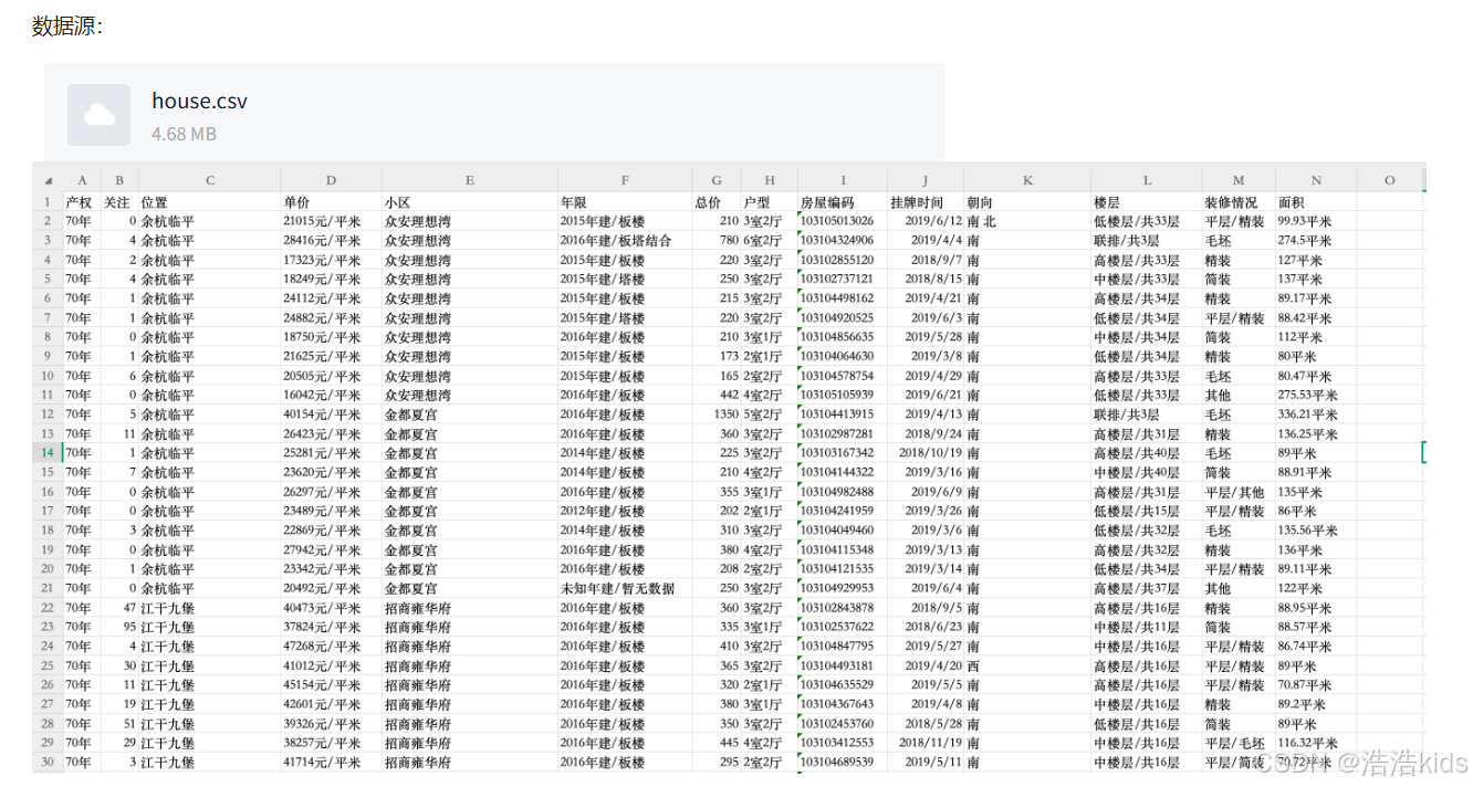
❤️理解
👌在R语言的read.csv函数中,header参数是一个逻辑值(TRUE或FALSE),用于指示数据文件的第一行是否包含变量名(即列名)。如果header=TRUE(默认值),则read.csv函数会将第一行作为列名,并且数据从第二行开始读取。如果header=FALSE,则read.csv函数会将第一行视为数据,并自动生成列名(如V1, V2, V3...)。stringsAsFactors = FALSE表示不自动转换为因子。
r
data <- read.csv("D:/myTemp/homework/R/作业数据源/house.csv",header = TRUE,stringsAsFactors = FALSE)👌grepl在data$年限中搜索包含"未知年建"的行,对包含"未知年建"的行返回TRUE,则 !grepl 对返回的结果取反后,包含的为FALSE,即删除了包含该文本的行。
r
# 删除"年限"列值包含"未知年建"的行
data <- data[!grepl("未知年建",data$年限),]
👌即保留小于等于3000的
r
# 2)异常值处理
# 删除总价大于3000万元的行
data <- data[data$总价 <= 3000,]👌substr的参数是substr(数据源,开始,结尾),第二个参数nchar(data$装修情况) - 1定位到倒数第二个字符,最后一个参数的nchar(data$装修情况)计算出字符总长度,因为在R语言中,字符串的索引是从1开始的,所以总长度也就是字符串最后一个字符的索引,substr函数不可省略第三个参数,如果你确实想省略第三个参数,可以使用substring()函数。
r
# 4)"装修情况"、"面积"列处理
# 取装修情况列的最后2个字符
data$装修情况 <- substr(data$装修情况,nchar(data$装修情况) - 1,nchar(data$装修情况))
👌gsub函数的参数为gsub(要被替换,替换后,数据源),替换后为""即相当于删除
r
# 去除面积列的"平米"字符并转换为数值型
data$面积 <- as.numeric(gsub("平米","",data$面积))
❤️完整代码
r
# 读取数据
data <- read.csv("D:/myTemp/homework/R/作业数据源/house.csv",header = TRUE,stringsAsFactors = FALSE)
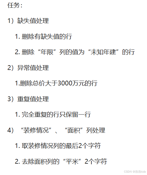
# 1)缺失值处理
# 删除有缺失值的行
data <- na.omit(data)
# 删除"年限"列值包含"未知年建"的行
data <- data[!grepl("未知年建",data$年限),]
# 2)异常值处理
# 删除总价大于3000万元的行
data <- data[data$总价 <= 3000,]
# 3)重复值处理
# 完全重复的行只保留一行
data <- unique(data)
# 4)"装修情况"、"面积"列处理
# 取装修情况列的最后2个字符
data$装修情况 <- substr(data$装修情况,nchar(data$装修情况) - 1,nchar(data$装修情况))
# 去除面积列的"平米"字符并转换为数值型
data$面积 <- as.numeric(gsub("平米","",data$面积))
# 查看处理后的数据结构
str(data)模型参数优化

r
rm(list = ls())
library(caret)
library(gbm)
library(Metrics)
car <- read.csv("D:/myTemp/homework/R/作业数据源/二手车(已处理缺失值、重复值).csv")
set.seed(1234)
num.idx <- sapply(car, is.numeric)
car_num <- car[, num.idx]
# 分离特征和目标变量
y <- car_num$售价
X <- subset(car_num, select = -售价)
# 划分训练集(占80%)和测试集(占20%)
set.seed(1234)
train_id <- createDataPartition(y, p = 0.8, list = FALSE)
X_train <- X[train_id,]
y_train <- y[train_id]
X_test <- X[-train_id,]
y_test <- y[-train_id]
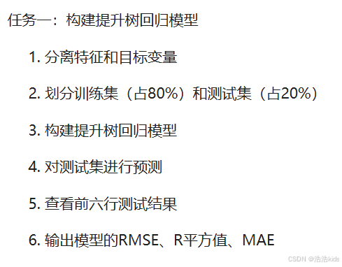
# 任务一:构建提升树回归模型
gbm_model <- gbm.fit(x = as.matrix(X_train),y = y_train,distribution = "gaussian",
n.trees = 3000,interaction.depth = 4,shrinkage = 0.01,
bag.fraction = 0.8,verbose = FALSE)
pred_gbm <- predict(gbm_model, newdata = as.matrix(X_test), n.trees = 3000)
head(pred_gbm)
rmse_gbm <- rmse(y_test, pred_gbm)
r2_gbm <- R2(pred_gbm, y_test)
mae_gbm <- mae(y_test, pred_gbm)
metrics <- data.frame(RMSE = rmse_gbm,Rsquared = r2_gbm,MAE = mae_gbm)
print("提升树回归模型结果:")
print(metrics)
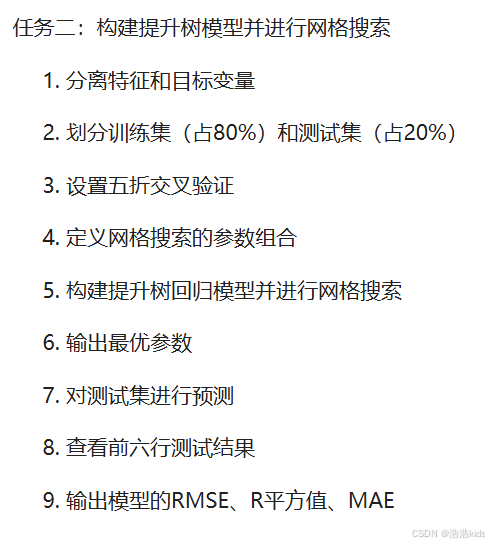
# 任务二:构建提升树模型并进行网格搜索
# 设置五折交叉验证
ctrl <- trainControl(method = "cv", number = 5)
# 定义网格搜索的参数组合
gbm_grid <- expand.grid(n.trees = c(1000, 2000, 3000),interaction.depth = c(3, 4, 5),
shrinkage = c(0.01, 0.05),n.minobsinnode = 10)
# 构建提升树回归模型并进行网格搜索
gbm_cv <- train(x = as.matrix(X_train),y = y_train,
method = "gbm",distribution = "gaussian",trControl = ctrl,
tuneGrid = gbm_grid,verbose = FALSE)
# 输出最优参数
gbm_cv$bestTune
# 对测试集进行预测
pred_cv <- predict(gbm_cv, newdata = as.matrix(X_test))
# 查看前六行测试结果
head(pred_cv)
# 输出模型的RMSE、R平方值、MAE
rmse_gbm <- rmse(y_test, pred_gbm)
r2_gbm <- R2(pred_gbm, y_test)
mae_gbm <- mae(y_test, pred_gbm)
metrics <- data.frame(RMSE = rmse_gbm,Rsquared = r2_gbm,MAE = mae_gbm)
print("网格搜索后结果:")
print(metrics)期中编程题
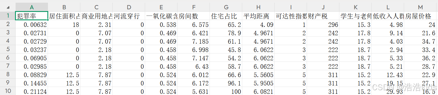
数据源:boston_house_prices.csv
字段介绍:犯罪率、居住面积占比、商业用地占比、河流穿行、一氧化氮含量、房间数、住宅占比、平均距离、可达性指数、财产税、学生与老师占比、低收入人群、房屋价格(千美元)。
1、读取数据,提取房屋价格数据,绘制房屋价格分布直方图。
r
library(tidyverse)
library(plotly)
data <- read.csv('D:/myTemp/homework/R/作业数据源/boston_house_prices.csv',fileEncoding = "GBK")
data
plot_ly(data, x = ~房屋价格, type = 'histogram') %>%
layout(title = list(text = '房屋价格分布', y = 0.99),
       xaxis = list(title = "房屋价格(千美元)"),
yaxis = list(title = "数量")) 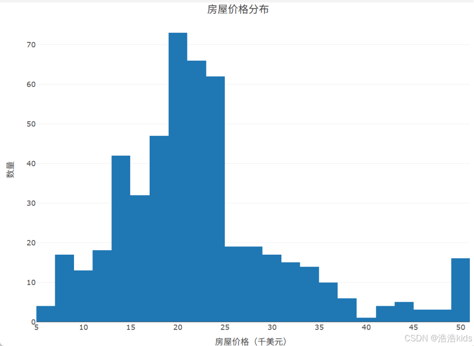
2、提取河流穿行与房屋价格数据,绘制河流穿行与房屋价格关系箱线图。
r
plot_ly(data, x = ~河流穿行, y = ~房屋价格, type = 'box') %>%
layout(title = list(text = '河流穿行与房屋价格关系', y = 0.99),
       xaxis = list(title = "河流穿行"),
yaxis = list(title = "房屋价格(千美元)")) 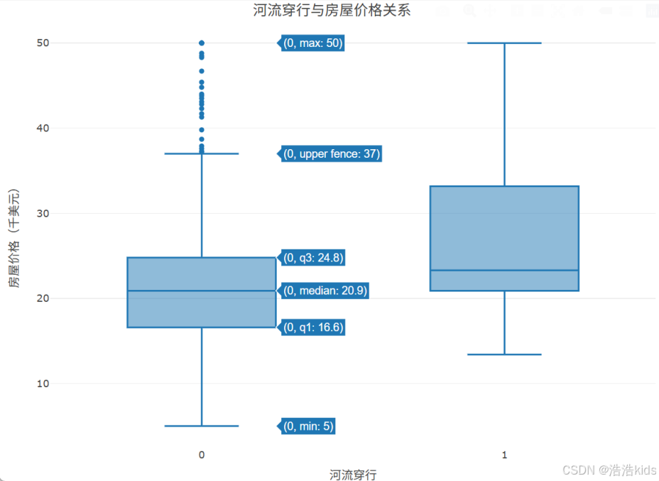
3、提取低收入人群与房屋价格数据,绘制低收入人群与房屋价格关系散点图。
r
plot_ly(data, x = ~低收入人群, y = ~房屋价格, type = 'scatter') %>%
add_lines(y = fitted(lm(房屋价格 ~ 低收入人群, data = data))) %>%
layout(title = list(text = '低收入人群与房屋价格关系', y = 0.99),
       xaxis = list(title = "低收入人群"),
yaxis = list(title = "房屋价格(千美元)")) 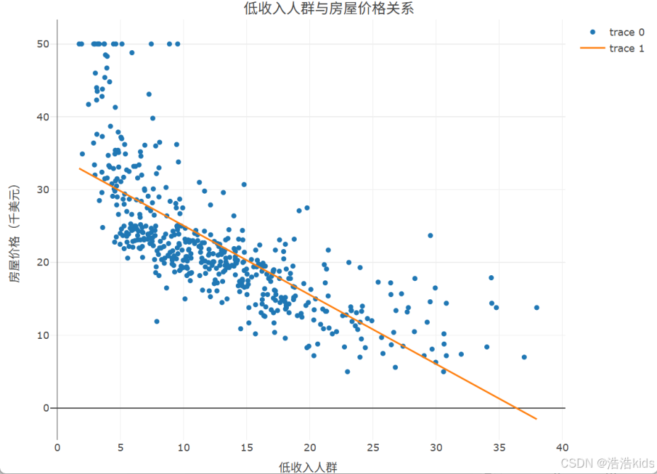
4、统计不同可达性指数房屋的平均价格,绘制可达性指数与房屋价格关系条形图。
r
price_keda <- data %>%
  group_by(可达性指数) %>%
  summarise(平均价格 = mean(房屋价格))
price_keda
price_keda$可达性指数 <- factor(price_keda$可达性指数, levels = price_keda$可达性指数)
plot_ly(price_keda, x = ~平均价格, y = ~可达性指数, type = 'bar', orientation = "h") %>%
layout(title = list(text = '可达性指数与房屋价格关系', y = 0.99),
       xaxis = list(title = "房屋价格(千美元)"),
       yaxis = list(title = "可达性指数"))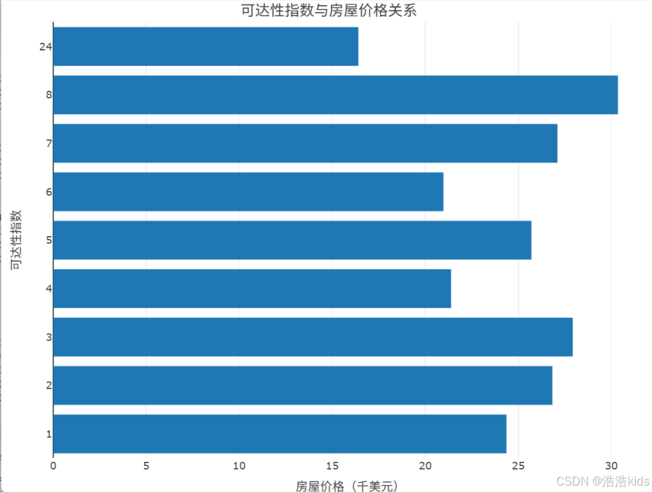
5、统计不同可达性指数房屋的数量,绘制不同可达性指数房屋数量占比环形图。
r
count_keda <- data %>%
  group_by(可达性指数) %>%
summarise(房屋数量 = n())
count_keda
plot_ly(count_keda, labels = ~可达性指数, values = ~房屋数量, type = 'pie', hole = 0.6) %>%
layout(title = list(text = '不同可达性指数房屋数量占比环形图', y = 0.99), showlegend = FALSE) 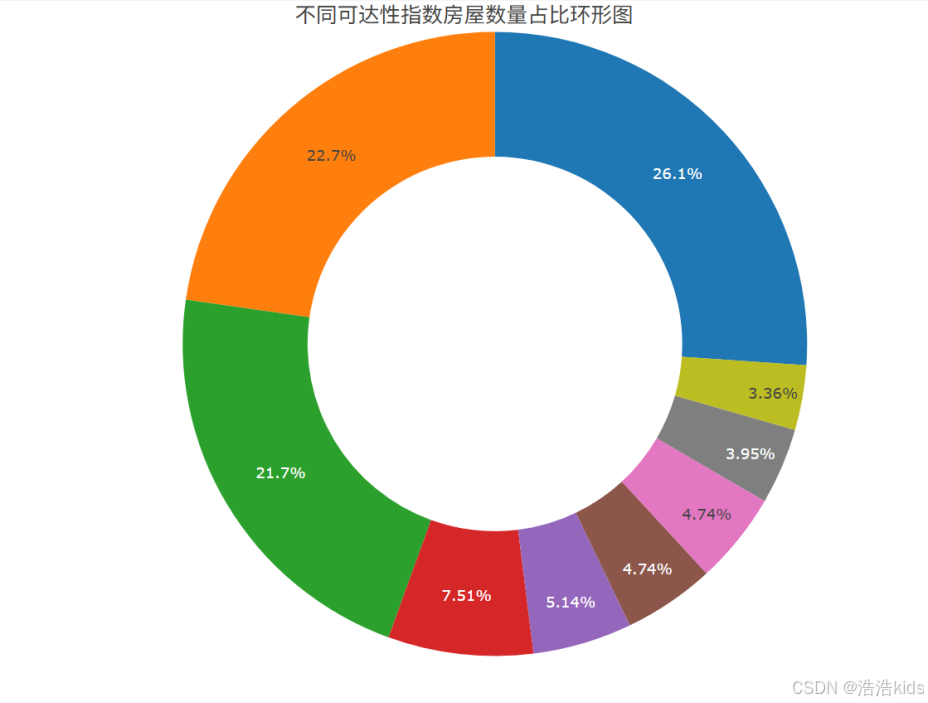
期末复习(二)
期末复习(一)是选择、填空、判断题~

整体介绍:根据杭州二手房的面积、位置、装修情况来预测价格(万元)。
数据源:杭州二手房.csv
1、读取数据,划分训练集(占80%)和测试集(占20%)。
2、构建线性回归模型,输出模型测试的结果、RMSE、R平方值、MAE。
3、构建决策树回归模型,输出模型测试的结果、RMSE、R平方值、MAE。
4、构建神经网络回归模型,输出模型测试的结果、RMSE、R平方值、MAE。
5、构建支持向量机回归模型,输出模型测试的结果、RMSE、R平方值、MAE。
r
rm(list = ls()) # 清空工作环境
library(caret) # 数据划分
library(rpart) # 决策树回归模型
library(nnet) # 神经网络回归模型
library(e1071) # 支持向量机回归模型
library(Metrics) # 计算RMSE、MAE

# 读取数据
house <- read.csv("D:/myTemp/homework/R/作业数据源/杭州二手房.csv")

# 取数值列
num.idx <- sapply(house, is.numeric)
house_num <- house[, num.idx]

# 分离特征和目标变量
y <- house_num$价格
X <- subset(house_num, select = -价格)

# 1. 划分训练集(占80%)和测试集(占20%)
set.seed(1234)
train_id <- createDataPartition(y, p = 0.8, list = FALSE)
train_data <- house_num[train_id,]
test_data <- house_num[-train_id,]

# 2、 构建线性回归模型,输出模型测试的结果、RMSE、R平方值、MAE。
lm_model <- lm(价格~.,data = train_data)
pred_lm <- predict(lm_model, newdata = test_data)

# 查看前六行测试结果
head(pred_lm)

# RMSE、R平方值、MAE
rmse_lm <- rmse(test_data$价格, pred_lm)
r2_lm <- caret::R2(test_data$价格,pred_lm)
mae_lm <- mae(test_data$价格, pred_lm)

metrics_lm <- data.frame(RMSE = rmse_lm,Rsquared = r2_lm,MAE = mae_lm)
print(metrics_lm)

# 3、构建决策树回归模型,输出模型测试的结果、RMSE、R平方值、MAE。
tree_model <- rpart(
  formula = 价格 ~ .,
  data = train_data,
  control = rpart.control(maxdepth = 3, minsplit = 10)
)
pred_tree <- predict(tree_model, newdata = test_data)

# 查看前六行测试结果
head(pred_tree)

# RMSE、R平方值、MAE
rmse_tree <- rmse(test_data$价格, pred_tree)
r2_tree <- caret::R2(test_data$价格,pred_tree)
mae_tree <- mae(test_data$价格, pred_tree)

metrics_tree <- data.frame(RMSE = rmse_tree,Rsquared = r2_tree,MAE = mae_tree)
print(metrics_tree)

# 4、构建神经网络回归模型,输出模型测试的结果、RMSE、R平方值、MAE。
nn_model <- nnet(
  formula = 价格 ~ .,          # 正确的公式格式
  data = train_data,           # 使用训练集数据
  size = 5,                    # 隐藏层神经元数量
  maxit = 1000,                # 最大迭代次数
  decay = 0.01,                # 权重衰减(正则化)参数
  linout = TRUE,               # 使用线性输出层
  trace = FALSE                # 不显示训练过程
)
pred_nn <- predict(nn_model, newdata = test_data)

# 查看前六行测试结果
head(pred_nn)

# RMSE、R平方值、MAE
rmse_nn <- rmse(test_data$价格, pred_nn)
r2_nn <- caret::R2(test_data$价格,pred_nn)
mae_nn <- mae(test_data$价格, pred_nn)

metrics_nn <- data.frame(RMSE = rmse_nn,Rsquared = r2_nn,MAE = mae_nn)
print(metrics_nn)

# 5、构建支持向量机回归模型,输出模型测试的结果、RMSE、R平方值、MAE。
svm_model <- svm(
  formula = 价格 ~ .,
  data = train_data,
  kernel = "radial",
  cost = 1,  # 惩罚参数
  gamma = 0.25,  # 核函数参数
  probability = TRUE  # 允许输出概率
)

pred_svm <- predict(svm_model, newdata = test_data)

# 查看前六行测试结果
head(pred_svm)

# RMSE、R平方值、MAE
rmse_svm <- rmse(test_data$价格, pred_svm)
r2_svm <- caret::R2(test_data$价格,pred_svm)
mae_svm <- mae(test_data$价格, pred_svm)

metrics_svm <- data.frame(RMSE = rmse_svm,Rsquared = r2_svm,MAE = mae_svm)
print(metrics_svm)