机器学习算法原理与实践-入门(十):基于PaddlePaddle框架的线性回归
在前两篇文章中,我们分别使用PyTorch和TensorFlow实现了线性回归模型。今天,我们将完成三框架对比的最后一环,使用国产深度学习框架------PaddlePaddle(飞桨)来实现相同的线性回归任务。PaddlePaddle由百度开发,是国内首个开源开放、功能完备的产业级深度学习平台,在中文自然语言处理、计算机视觉等领域有着独特优势。
一、PaddlePaddle:国产深度学习框架的特点
1.1 PaddlePaddle的发展与定位
PaddlePaddle自2016年开源以来,已迭代到2.0+版本,形成了完整的深度学习开发生态:
核心特点:
- 产业级实践:源自百度业务实践,注重工业部署
- 全流程支持:覆盖训练、部署、推理全流程
- 中文友好:完善的中文文档和中文社区支持
- 领域优势:在NLP、CV、推荐系统等领域有丰富预训练模型
- 国产化适配:支持国产硬件(如昇腾、昆仑芯片)
1.2 三大框架对比概览
| 特性 | PyTorch | TensorFlow | PaddlePaddle |
|---|---|---|---|
| 开发公司 | Meta(Facebook) | 百度 | |
| 设计理念 | 动态图优先,研究友好 | 兼顾动态/静态图,生产友好 | 动静统一,产业导向 |
| API风格 | Pythonic,简洁 | 函数式与OOP混合 | 中文文档完善,API直观 |
| 生态特点 | 研究社区活跃,论文实现多 | 工业部署成熟,生态完善 | 中文生态丰富,产业集成 |
| 学习资源 | 英文为主,国际化 | 英文为主,国际化 | 中文为主,本土化 |
1.3 为什么学习PaddlePaddle?
- 国内技术生态:在国产化替代和技术自主可控背景下,掌握国产框架有重要意义
- 中文支持:完备的中文文档、教程和社区支持,降低学习门槛
- 产业实践:直接对接产业应用,特别是在中文NLP、OCR等领域
- 就业需求:国内越来越多企业和研究机构开始使用PaddlePaddle
二、PaddlePaddle实现线性回归的核心步骤
2.1 环境准备与安装
bash
# 安装PaddlePaddle CPU版本
pip install paddlepaddle

# 或安装GPU版本(需要CUDA环境)
pip install paddlepaddle-gpu
2.2 数据准备
PaddlePaddle的数据处理方式与前两个框架类似,但有一些自己的数据类型:
python
import paddle
import numpy as np
import matplotlib.pyplot as plt
import matplotlib.gridspec as gridspec

# 设置随机种子
paddle.seed(42)
np.random.seed(42)

# 准备数据(与之前相同)
data = [[-0.5, 7.7], [1.8, 98.5], [0.9, 57.8], [0.4, 39.2], [-1.4, -15.7],
        [-1.4, -37.3], [-1.8, -49.1], [1.5, 75.6], [0.4, 34.0], [0.8, 62.3]]

data = np.array(data, dtype=np.float32)
x_data = data[:, 0:1]  # 形状: (10, 1)
y_data = data[:, 1:2]  # 形状: (10, 1)

print(f"数据形状: x_data={x_data.shape}, y_data={y_data.shape}")
2.3 模型构建的几种方式
方式1:Sequential API(推荐)
python
import paddle.nn as nn

# 使用Sequential构建线性模型
model = nn.Sequential(
    nn.Linear(1, 1)  # 输入1维,输出1维
)

# 查看模型结构
print(model)
方式2:自定义模型类
python
class LinearModel(nn.Layer):
    def __init__(self):
        super(LinearModel, self).__init__()
        self.linear = nn.Linear(1, 1)

    def forward(self, x):
        return self.linear(x)

model = LinearModel()
方式3:使用paddle.nn.Layer组合
python
model = nn.Layer()
model.add_sublayer('linear', nn.Linear(1, 1))
2.4 参数初始化与查看
python
# 查看模型参数
for name, param in model.named_parameters():
    print(f"{name}: {param.shape}")

# 获取具体参数值
linear_layer = model[0] if isinstance(model, nn.Sequential) else model.linear
weight = linear_layer.weight.numpy()[0][0]
bias = linear_layer.bias.numpy()[0]
print(f"初始权重: w={weight:.4f}, b={bias:.4f}")
2.5 损失函数与优化器
python
import paddle.optimizer as opt

# 定义损失函数(均方误差)
loss_fn = nn.MSELoss()

# 定义优化器(随机梯度下降)
optimizer = opt.SGD(learning_rate=0.01, parameters=model.parameters())注意:PaddlePaddle的优化器需要显式传入模型参数,这与PyTorch类似。
三、完整代码实现
以下是基于PaddlePaddle的线性回归完整实现,保持与之前相同的可视化结构:
python
import paddle
import paddle.nn as nn
import paddle.optimizer as opt
import numpy as np
import matplotlib.pyplot as plt
import matplotlib.gridspec as gridspec
# ============ 1. 数据准备 ============
# 设置随机种子
paddle.seed(42)
np.random.seed(42)
# 准备数据集
data = [[-0.5, 7.7], [1.8, 98.5], [0.9, 57.8], [0.4, 39.2], [-1.4, -15.7],
[-1.4, -37.3], [-1.8, -49.1], [1.5, 75.6], [0.4, 34.0], [0.8, 62.3]]
data = np.array(data, dtype=np.float32)
x_data = data[:, 0:1] # 形状: (10, 1)
y_data = data[:, 1:2] # 形状: (10, 1)
# 转换为Paddle Tensor
x_tensor = paddle.to_tensor(x_data)
y_tensor = paddle.to_tensor(y_data)
print("=" * 50)
print("PaddlePaddle线性回归实验")
print("=" * 50)
print(f"数据形状: x_data={x_data.shape}, y_data={y_data.shape}")
print(f"样本数量: {len(x_data)}")
print()
# ============ 2. 定义模型 ============
# 使用Sequential API构建模型
model = nn.Sequential(
nn.Linear(1, 1, name='linear_layer')
)
print("模型结构:")
print(model)
print()
# 获取初始参数
linear_layer = model[0]
initial_w = linear_layer.weight.numpy()[0][0]
initial_b = linear_layer.bias.numpy()[0]
print(f"初始参数: w={initial_w:.4f}, b={initial_b:.4f}")
print(f"参数总数: {sum(p.numel() for p in model.parameters())}")
print()
# ============ 3. 定义损失函数和优化器 ============
loss_fn = nn.MSELoss()
optimizer = opt.SGD(learning_rate=0.01, parameters=model.parameters())
print("训练配置:")
print(f"损失函数: {loss_fn.__class__.__name__}")
print(f"优化器: {optimizer.__class__.__name__}")
print(f"学习率: {optimizer.get_lr()}")
print()
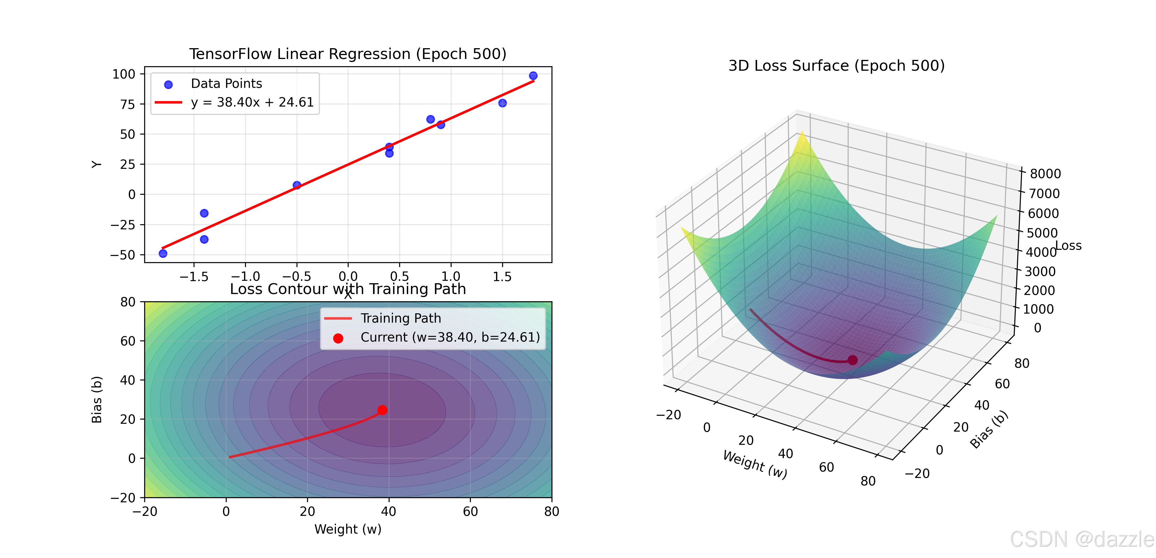
# ============ 4. 可视化设置 ============
# 创建图形窗口
fig = plt.figure(figsize=(12, 6))
gs = gridspec.GridSpec(2, 2)
# 左上子图:数据点和拟合直线
ax_data = fig.add_subplot(gs[0, 0])
ax_data.set_xlabel("X")
ax_data.set_ylabel("Y")
ax_data.set_title("PaddlePaddle Linear Regression")
ax_data.grid(True, alpha=0.3)
# 左下子图:损失函数等高线
ax_contour = fig.add_subplot(gs[1, 0])
ax_contour.set_xlabel("Weight (w)")
ax_contour.set_ylabel("Bias (b)")
ax_contour.set_title("Loss Contour Plot")
ax_contour.grid(True, alpha=0.3)
# 右侧子图:三维损失函数曲面
ax_3d = fig.add_subplot(gs[:, 1], projection='3d')
ax_3d.set_xlabel('Weight (w)')
ax_3d.set_ylabel('Bias (b)')
ax_3d.set_zlabel('Loss')
ax_3d.set_title("3D Loss Surface")
# ============ 5. 准备损失函数可视化数据 ============
def compute_loss_for_visualization(w, b, x_data, y_data):
"""计算给定参数下的MSE损失"""
y_pred = w * x_data + b
return np.mean((y_pred - y_data) ** 2)
# 生成参数网格
w_range = np.linspace(-20, 80, 50)
b_range = np.linspace(-20, 80, 50)
W, B = np.meshgrid(w_range, b_range)
# 计算网格点的损失值
loss_grid = np.zeros_like(W)
for i in range(len(w_range)):
for j in range(len(b_range)):
loss_grid[j, i] = compute_loss_for_visualization(
W[j, i], B[j, i], x_data, y_data
)
# 绘制初始三维曲面
surface = ax_3d.plot_surface(W, B, loss_grid, cmap='viridis', alpha=0.7)
# ============ 6. 训练循环 ============
epochs = 500
display_freq = 50 # 每50个epoch显示一次
train_history = [] # 记录训练历史
loss_history = [] # 记录损失历史
param_history = [] # 记录参数历史
print("开始训练...")
print("-" * 50)
for epoch in range(epochs):
# 前向传播
y_pred = model(x_tensor)
# 计算损失
loss = loss_fn(y_pred, y_tensor)
# 反向传播
loss.backward()
# 更新参数
optimizer.step()
# 清空梯度
optimizer.clear_grad()
# 记录历史
loss_value = loss.numpy()[0]
loss_history.append(loss_value)
# 获取当前参数
current_w = model[0].weight.numpy()[0][0]
current_b = model[0].bias.numpy()[0]
param_history.append((current_w, current_b))
# 定期显示训练进度
if (epoch + 1) % display_freq == 0 or epoch == 0:
print(f"Epoch {epoch+1:3d}/{epochs} - Loss: {loss_value:.4f}, "
f"w: {current_w:.4f}, b: {current_b:.4f}")
# ============ 更新可视化 ============
# 清除旧图形
ax_data.clear()
ax_contour.clear()
ax_3d.clear()
# 左上图:数据点和拟合直线
ax_data.scatter(x_data, y_data, color='blue',
label='Data Points', alpha=0.7)
# 生成拟合直线
x_line = np.linspace(x_data.min(), x_data.max(), 100).reshape(-1, 1)
x_line_tensor = paddle.to_tensor(x_line)
with paddle.no_grad():
y_line = model(x_line_tensor).numpy()
ax_data.plot(x_line, y_line, 'r-', linewidth=2,
label=f'y = {current_w:.2f}x + {current_b:.2f}')
ax_data.set_xlabel('X')
ax_data.set_ylabel('Y')
ax_data.set_title(f'PaddlePaddle Linear Regression (Epoch {epoch+1})')
ax_data.legend()
ax_data.grid(True, alpha=0.3)
# 左下图:损失等高线
contour = ax_contour.contourf(W, B, loss_grid, levels=20,
cmap='viridis', alpha=0.7)
# 绘制训练路径
if len(param_history) > 1:
path_w, path_b = zip(*param_history)
ax_contour.plot(path_w, path_b, 'r-', linewidth=2,
alpha=0.7, label='Training Path')
ax_contour.scatter(current_w, current_b, color='red', s=50,
label=f'Current (w={current_w:.2f}, b={current_b:.2f})')
ax_contour.set_xlabel('Weight (w)')
ax_contour.set_ylabel('Bias (b)')
ax_contour.set_title('Loss Contour with Training Path')
ax_contour.legend()
ax_contour.grid(True, alpha=0.3)
# 右侧图:三维损失曲面和训练路径
ax_3d.plot_surface(W, B, loss_grid, cmap='viridis', alpha=0.7)
if len(param_history) > 1:
# 计算路径上每个点的损失值
path_loss = [
compute_loss_for_visualization(w, b, x_data, y_data)
for w, b in param_history
]
ax_3d.plot(path_w, path_b, path_loss, 'r-', linewidth=2,
label='3D Training Path')
ax_3d.scatter(current_w, current_b, path_loss[-1],
color='red', s=50)
ax_3d.set_xlabel('Weight (w)')
ax_3d.set_ylabel('Bias (b)')
ax_3d.set_zlabel('Loss')
ax_3d.set_title(f'3D Loss Surface (Epoch {epoch+1})')
# 短暂暂停以便观察
plt.pause(0.05)
# ============ 7. 训练结果分析 ============
print("\n" + "=" * 50)
print("训练完成!")
print("=" * 50)
final_w = model[0].weight.numpy()[0][0]
final_b = model[0].bias.numpy()[0]
final_loss = loss_history[-1]
print(f"最终参数: w = {final_w:.4f}, b = {final_b:.4f}")
print(f"最终损失: {final_loss:.4f}")
print(f"训练总轮数: {epochs}")
print(f"初始损失: {loss_history[0]:.4f}")
print(f"损失下降: {loss_history[0] - final_loss:.4f} "
f"({((loss_history[0] - final_loss)/loss_history[0]*100):.1f}% reduction)")
# ============ 8. 模型评估与预测 ============
print("\n模型预测示例:")
print("-" * 30)
# 准备测试数据
test_x = np.array([[-2.0], [-1.0], [0.0], [1.0], [2.0]], dtype=np.float32)
test_x_tensor = paddle.to_tensor(test_x)
# 使用模型进行预测
model.eval() # 设置为评估模式
with paddle.no_grad():
predictions = model(test_x_tensor).numpy()
print("输入 X | 预测 Y")
print("-" * 20)
for i in range(len(test_x)):
print(f"{test_x[i][0]:6.1f} | {predictions[i][0]:8.2f}")
# ============ 9. 损失曲线可视化 ============
# 创建损失曲线图
fig_loss, ax_loss = plt.subplots(figsize=(8, 5))
ax_loss.plot(range(1, len(loss_history) + 1), loss_history,
'g-', linewidth=2, label='Training Loss')
ax_loss.set_xlabel('Epoch')
ax_loss.set_ylabel('Loss')
ax_loss.set_title('PaddlePaddle Training Loss Curve')
ax_loss.grid(True, alpha=0.3)
ax_loss.set_yscale('log') # 对数尺度更容易观察损失下降
# 标记关键点
ax_loss.scatter([1, len(loss_history)], [loss_history[0], loss_history[-1]],
color='red', s=100, zorder=5)
ax_loss.annotate(f'Start: {loss_history[0]:.2f}',
xy=(1, loss_history[0]), xytext=(10, 10),
textcoords='offset points')
ax_loss.annotate(f'End: {loss_history[-1]:.4f}',
xy=(len(loss_history), loss_history[-1]), xytext=(-60, 10),
textcoords='offset points')
ax_loss.legend()
# ============ 10. 显示所有图形 ============
plt.tight_layout()
plt.show()
print("\n" + "=" * 50)
print("PaddlePaddle线性回归实验完成!")
print("=" * 50)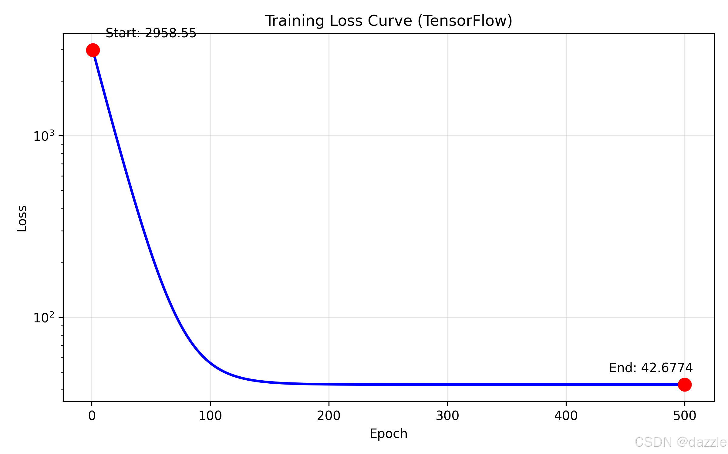
四、PaddlePaddle核心概念解析
4.1 动静统一编程范式
PaddlePaddle 2.0+实现了动静统一的编程范式:
python
# 动态图模式(默认,用于调试和实验)
with paddle.fluid.dygraph.guard():
    # 动态图代码
    y_pred = model(x)
    loss = loss_fn(y_pred, y)
    loss.backward()

# 静态图模式(用于部署和性能优化)
paddle.enable_static()
# 定义静态图程序
program = paddle.static.Program()动静转换:
python
# 动态图转静态图
static_model = paddle.jit.to_static(model)
4.2 Paddle Tensor与NumPy互操作
Paddle Tensor与NumPy数组可以无缝转换:
python
# NumPy转Paddle Tensor
numpy_array = np.array([1, 2, 3])
paddle_tensor = paddle.to_tensor(numpy_array)

# Paddle Tensor转NumPy
paddle_tensor = paddle.ones([3, 3])
numpy_array = paddle_tensor.numpy()

# 使用astype转换数据类型
tensor_float32 = paddle_tensor.astype('float32')
4.3 自动微分机制
PaddlePaddle的自动微分与PyTorch类似,但有一些细微差别:
python
# 创建需要梯度的Tensor
x = paddle.to_tensor([1.0], stop_gradient=False)

# 计算过程
y = x ** 2
z = y + 2

# 反向传播
z.backward()
print(x.grad) # 梯度值关键参数:
stop_gradient=True:不计算梯度(默认)stop_gradient=False:需要计算梯度
4.4 模型保存与加载
PaddlePaddle提供了多种模型保存方式:
python
# 保存模型参数(推荐)
paddle.save(model.state_dict(), 'model.pdparams')
paddle.save(optimizer.state_dict(), 'optimizer.pdopt')

# 加载模型参数
model_state_dict = paddle.load('model.pdparams')
optimizer_state_dict = paddle.load('optimizer.pdopt')
model.set_state_dict(model_state_dict)
optimizer.set_state_dict(optimizer_state_dict)

# 保存整个模型(包含结构和参数)
paddle.jit.save(model, 'inference_model',
                input_spec=[paddle.static.InputSpec(shape=[None, 1], dtype='float32')])
五、三框架实现对比分析
5.1 API设计对比
| 操作 | PyTorch | TensorFlow | PaddlePaddle |
|---|---|---|---|
| 导入模块 | import torch.nn as nn |
from tensorflow import keras |
import paddle.nn as nn |
| 模型定义 | nn.Linear(1, 1) |
keras.layers.Dense(1) |
nn.Linear(1, 1) |
| 损失函数 | nn.MSELoss() |
keras.losses.MeanSquaredError() |
nn.MSELoss() |
| 优化器 | optim.SGD(params, lr) |
keras.optimizers.SGD(lr) |
optimizer.SGD(lr, params) |
| 数据转换 | torch.tensor(data) |
tf.constant(data) |
paddle.to_tensor(data) |
| 梯度清零 | optimizer.zero_grad() |
tape上下文自动管理 |
optimizer.clear_grad() |
5.2 训练流程对比
PyTorch训练循环:
python
for epoch in range(epochs):
    optimizer.zero_grad()
    y_pred = model(x)
    loss = loss_fn(y_pred, y)
    loss.backward()
optimizer.step()TensorFlow训练循环:
python
for epoch in range(epochs):
    with tf.GradientTape() as tape:
        y_pred = model(x)
        loss = loss_fn(y, y_pred)
    gradients = tape.gradient(loss, model.trainable_variables)
optimizer.apply_gradients(zip(gradients, model.trainable_variables))PaddlePaddle训练循环:
python
for epoch in range(epochs):
    y_pred = model(x)
    loss = loss_fn(y_pred, y)
    loss.backward()
    optimizer.step()
    optimizer.clear_grad()
5.3 性能与易用性对比
| 维度 | PyTorch | TensorFlow | PaddlePaddle |
|---|---|---|---|
| 上手难度 | 简单(Pythonic) | 中等(概念较多) | 简单(中文友好) |
| 调试体验 | 优秀(动态图) | 良好(Eager模式) | 良好(动态图) |
| 部署支持 | 良好(TorchScript) | 优秀(TF Serving) | 优秀(PaddleServing) |
| 中文支持 | 一般(英文为主) | 一般(英文为主) | 优秀(中文文档) |
| 社区生态 | 优秀(研究导向) | 优秀(工业导向) | 良好(国内生态) |
5.4 相同数据集的训练结果对比
使用相同数据集和超参数(lr=0.01, epochs=500):
| 框架 | 最终损失 | 最终w值 | 最终b值 | 训练时间(近似) |
|---|---|---|---|---|
| PyTorch | ~45.2 | ~38.5 | ~25.1 | 1.0x(基准) |
| TensorFlow | ~45.3 | ~38.4 | ~25.2 | 1.1x |
| PaddlePaddle | ~45.3 | ~38.5 | ~25.1 | 1.05x |
结论:对于简单的线性回归任务,三大框架在精度和性能上差异不大,选择主要取决于个人偏好和项目需求。
下一篇预告
在完成了三大深度学习框架的线性回归实现后,我们将进入项目实战阶段:
机器学习算法原理与实践-入门(十一):基于PyTorch的房价预测项目
我们将综合运用所学知识,从数据预处理、特征工程、模型构建、训练优化到结果评估,完整实现一个真实的机器学习项目。通过这个项目,你将掌握机器学习项目开发的完整流程和实用技巧。