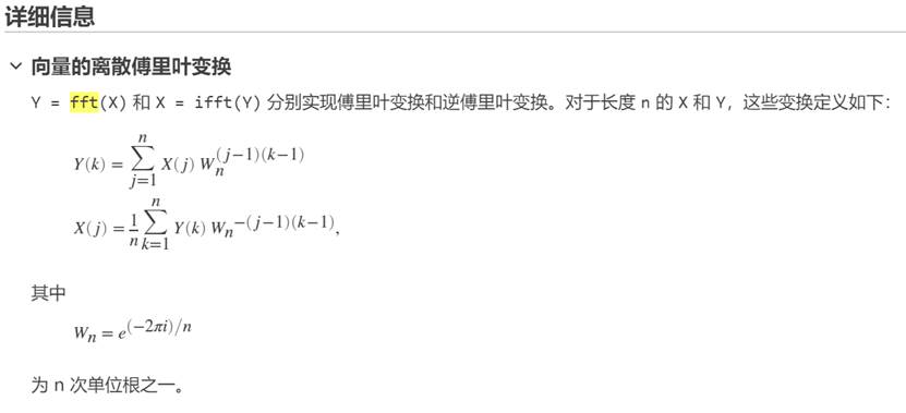
FFT Spectrum and Spectral Densities -- Same Data, Different Scaling
快速傅里叶变换频谱与噪声功率频谱密度 ------ 相同的数据,不同的缩放
邓敏 2025 1 8
PSD 和均方差的比较
Fast Fourier Transform (FFT) analysis, which converts signals from the time domain to their frequency domain equivalent, is incredibly useful in audio test. Precise estimates of many fundamental audio quality metrics such as frequency, level, harmonic distortion, intermodulation distortion, crosstalk, etc., can all be derived from FFT analysis. In fact, all but a few of the hundreds of results available in Sequence Mode in the APx500 software are derived from FFT analysis.
Most users are familiar with the FFT Spectrum result, typically used for analyzing signals with discrete frequency components (like sine waves). But many may be less familiar with the Power Spectral Density and Amplitude Spectral Density results, which are typically used when analyzing noise. This post explains the difference between these spectral density results and the more commonly used FFT Spectrum.
快速傅里叶变换(FFT)分析将信号从时域转换为其频域等效形式,在音频测试中极为有用。许多基本音频质量指标的精确估计,如频率、电平、谐波失真、互调失真、串扰等,都可以从FFT分析中得出。事实上,APx500软件序列模式中可用的数百个结果中,除了少数几个外,都是从FFT分析中得出的。 大多数用户都熟悉FFT频谱结果,通常用于分析具有离散频率成分的信号(如正弦波)。但许多人可能不太熟悉功率谱密度和振幅谱密度结果,这些结果通常用于分析噪声。本文解释了这些谱密度结果与更常用的FFT频谱之间的区别。
FFT Spectrum
For illustration purposes, Figure 1 shows a signal that contains both a discrete frequency component as well as a relatively high level of broad band noise. The noise was created by using a digital interface with dither applied at a bit depth of only 8 bits. The Scope (waveform, left) and the FFT Spectrum results (right) for this sine signal at 1125 Hz with a level of -20 dBFS (or 0.10 FS) are shown.
FFT 频谱
为了说明,图1展示了一个信号,它既包含离散频率成分,又包含相对较高的宽带噪声水平。噪声是通过使用数字接口,并在仅8位比特深度下应用抖动而产生的。图中显示了这个1125赫兹、电平为-20分贝满量程(或0.10满量程)的正弦信号的示波器(波形,左侧)和FFT频谱结果(右侧)。
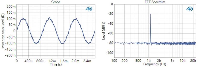
Figure 1. Waveform and 16k FFT Spectrum of a 48 kHz Fs digital sine signal with 8-bit dither (level = -20 dBFS; frequency = 1125 Hz).
图1. 采样频率为48千赫兹、采用8位抖动的数字正弦信号的波形和16k FFT频谱(电平=-20分贝满量程;频率=1125赫兹)。
The FFT Spectrum result (sometimes called the linear spectrum or rms spectrum) is derived from the FFT auto-spectrum, with the spectrum being scaled to represent the rms level at each frequency. As a result, the FFT Spectrum of a pure sine contains a peak at the frequency of the sine signal with amplitude equal to its rms level. For example, the peak in the FFT Spectrum in Figure 1 is exactly the expected signal level of -20 dBFS. The FFT Spectrum is ideally suited to analyzing signals with discrete components or tones.
But what if we're interested in quantifying the level of noise in this signal? From a casual observation of the spectrum in Figure 1, we might be tempted to say that "the noise floor in this measurement is at -80 dBFS", or "the signal-to-noise ratio is 60 dB". But these statements are wrong, because of the FFT spectrum's scaling for pure tones. This is obvious when you consider Figure 2, which shows the same signal as Figure 1 analyzed with three different FFT Length settings: 256, 16k and 1M points. Note that the peak remains at -20 dBFS, but the level of the apparent noise plateau decreases substantially as the number of FFT bins is increased.
FFT频谱结果(有时称为线性频谱或均方根频谱)是从FFT自谱中得出的,频谱被缩放以表示每个频率处的均方根电平。因此,纯正弦波的FFT频谱在其频率处包含一个峰值,其幅度等于其均方根电平。例如,图1中FFT频谱的峰值正是预期的信号电平-20分贝满量程。FFT频谱非常适合分析具有离散成分或音调的信号。 但如果我们对量化这个信号中的噪声电平感兴趣呢?从对图1中频谱的粗略观察来看,我们可能会被诱惑说"这个测量中的噪声地板在-80分贝满量程",或者"信噪比是60分贝"。但这些说法是错误的,因为FFT频谱对纯音调进行了缩放。当你考虑图2时,这一点就很明显了,图2显示了与图1相同的信号,但使用了三种不同的FFT长度设置:256点、16k点和1M点进行分析。请注意,峰值保持在-20分贝满量程,但随着FFT分箱数量的增加,看似噪声平台的电平大幅降低。
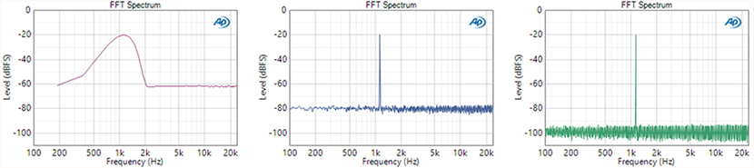
Figure 2. Linear FFT Spectra of the signal in Figure 1 with FFT Lengths of 256 (left), 16k (middle) and 1M samples (right). Note how the amplitude of the peak at 1125 Hz is constant, but the apparent noise plateau is reduced in level as the FFT Length increases.
图2. 图1中信号的线性FFT频谱,FFT长度分别为256(左侧)、16k(中间)和1M样本(右侧)。请注意,1125赫兹处峰值的幅度是恒定的,但随着FFT长度的增加,看似噪声平台的电平降低了。
The change in level of the noise plateau in Figure 2 is a result of the change in the FFT bin width. The noise is distributed over the entire frequency range, so the wider the FFT bins , the more noise each bin will contain. In fact, each time the bin width is doubled, the noise power per bin is also doubled, causing an increase of 3 dB in the rms level. With smoothing applied to the spectra in Figure 2, the apparent noise plateau is at -62, -80 and -98 dBFS for the FFT Length settings of 256, 16k and 1M, respectively (i.e., a change of -18 dB for each of the two steps). The increases in FFT Length from 256 to 16k and from 16k to 1M each correspond to the FFT bin width decreasing by a factor of 64, or 2^6. As a result, the rms noise level per bin decreases by 18 dB (i.e., 6 x 3 dB) in each case.
图2中噪声平台电平的变化是由于FFT分箱宽度的变化所致。噪声分布在整个频率范围内,因此FFT分箱越宽,每个分箱所包含的噪声就越多。实际上,每当分箱宽度加倍时,每个分箱中的噪声功率也会加倍,从而导致均方根电平增加3分贝。在图2的频谱中应用平滑处理后,对于256、16k和1M的FFT长度设置,看似噪声平台的电平分别为-62分贝满量程、-80分贝满量程和-98分贝满量程(即每一步变化-18分贝)。从256到16k以及从16k到1M的FFT长度增加,分别对应FFT分箱宽度减小64倍,即2的6次方。因此,在每种情况下,每个分箱的均方根噪声电平降低了18分贝(即6×3分贝)。
Spectral Density Results
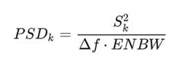
The Power Spectral Density is also derived from the FFT auto-spectrum, but it is scaled to correctly display the density of noise power (level squared in the signal), equivalent to the noise power at each frequency measured with a filter exactly 1 Hz wide. It has units of V2/Hz in the analog domain and FS2/Hz in the digital domain.
Figure 3 shows the Power Spectral Density results corresponding to the data of Figure 2. Note that the apparent noise plateau of the signal remains constant as the FFT bin width changes - however, the level of the discrete peak at 1125 Hz does change with FFT Length. In this case, a statement to the effect that "the noise floor in this signal is approximately 1 nV2/Hz" is correct.
谱密度结果
功率谱密度也是从FFT自谱中得出的,但它被缩放以正确显示噪声功率的密度(信号中的电平平方),相当于用一个正好1赫兹宽的滤波器在每个频率处测量到的噪声功率。在模拟域中,其单位为V²/Hz,在数字域中,其单位为FS²/Hz。 图3显示了与图2数据相对应的功率谱密度结果。请注意,随着FFT分箱宽度的变化,信号的看似噪声平台保持恒定------然而,1125赫兹处离散峰值的电平确实会随着FFT长度的变化而变化。在这种情况下,说"这个信号中的噪声地板大约为1纳伏²/赫兹"是正确的。
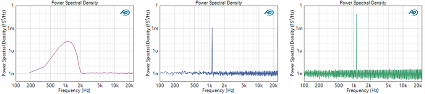
Figure 3. The same data as Figure 3 expressed as Power Spectral Density plots. Note how the noise plateau is constant, but the level of the peak increases with the FFT Length.
The Amplitude Spectral Density is also used to analyze noise signals. It has units of V/√ Hz in the analog domain and
FS/√ Hz in the digital domain. The Amplitude Spectral Density is simply the square root of the Power Spectral Density.
图3. 以功率谱密度图的形式表示与图3相同的数据。请注意,噪声平台是恒定的,但峰值的电平随着FFT长度的增加而增加。 振幅谱密度也用于分析噪声信号。在模拟域中,其单位为V/√Hz,在数字域中,其单位为FS/√Hz。振幅谱密度仅仅是功率谱密度的平方根。
FFT Windows and the Equivalent Noise Bandwidth (ENBW)
When conducting FFT analysis, typically, a window function is applied to the data before taking the Fourier transform to enforce the necessary condition that the signal is periodic within the sampled time block. Many types of FFT windows exist, and each has unique characteristics that offer certain application-dependent advantages and disadvantages. The default window used in APx500 software is the AP Equiripple window. Other common windows include the Hann and the Flat Top window.
A consequence of using an FFT window is that it spreads signal energy from each FFT bin into adjacent bins, effectively increasing the FFT bin width. The relative increase in bin width is characterized by a property known as the equivalent noise bandwidth (ENBW). Each window has a specific ENBW, which must be accounted for when scaling the FFT spectrum. For example, the ENBW of the AP Equiripple and Hann windows are 2.63 and 1.5, respectively. If no window is selected (sometimes called a Rectangular window), the ENBW is equal to 1.0.
The FFT Spectrum and the Power Spectral Density are related by the ENBW as shown in equation (1).
FFT 窗函数与等效噪声带宽( ENBW )
进行FFT分析时,通常会在进行傅里叶变换之前对数据应用一个窗函数,以满足信号在采样时间块内是周期性的必要条件。存在许多类型的FFT窗函数,每种窗函数都有其独特的特性,提供了某些与应用相关的优缺点。APx500软件中使用的默认窗函数是AP等波纹窗。其他常见的窗函数包括汉宁窗和平顶窗。 使用FFT窗函数的一个结果是,它会将每个FFT分箱中的信号能量扩散到相邻的分箱中,实际上增加了FFT分箱的宽度。分箱宽度的相对增加可以通过一个称为等效噪声带宽(ENBW)的属性来描述。每个窗函数都有一个特定的ENBW,在缩放FFT频谱时必须考虑这个属性。例如,AP等波纹窗和汉宁窗的ENBW分别为2.63和1.5。如果不选择窗函数(有时称为矩形窗),则ENBW等于1.0。 FFT频谱和功率谱密度通过ENBW相关联,如公式(1)所示。
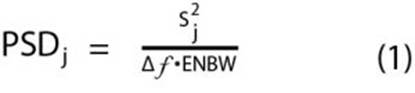
Where PSD represents the power spectral density, S represents the rms (or linear) spectrum, j is the FFT bin number and Δf is the FFT bin width.
其中PSD表示功率谱密度,S表示均方根(或线性)频谱,j是FFT分箱编号,Δf是FFT分箱宽度。
Level Calculations
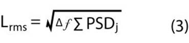
It's often required to calculate the rms level of noise within a specified frequency range. This can be done by integrating the FFT Spectrum or PSD between the frequencies of interest. Another common requirement is to estimate the rms level of a discrete frequency component, such as a harmonic. Typically, this is done by integrating the FFT over 3 FFT bins on either side of the bin containing the frequency of interest, to account for the spreading effect of the window. Equations (2) and (3) can be used to calculate rms level from the FFT Spectrum and PSD, where each summation is applied over the FFT bins spanning the frequency range of interest.
电平计算
通常需要计算在指定频率范围内噪声的均方根电平。这可以通过在感兴趣的频率之间对FFT频谱或PSD进行积分来完成。另一个常见需求是估计离散频率成分(如谐波)的均方根电平。通常,这是通过在包含感兴趣频率的分箱两侧各3个FFT分箱上对FFT进行积分来实现的,以考虑窗函数的扩散效应。公式(2)和(3)可用于从FFT频谱和PSD计算均方根电平,其中每个求和应用于跨越感兴趣频率范围的FFT分箱。
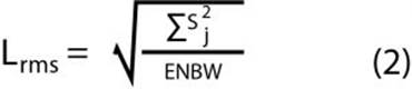
An advantage of using the PSD for this calculation (equation 3) is that it's not required to know which FFT window was used, because the ENBW is built into the PSD's scaling.
使用PSD进行此计算(公式3)的一个优势是,不需要知道使用了哪种FFT窗函数,因为等效噪声带宽(ENBW)已经包含在PSD的缩放中。
Reference
Heinzel, G., Rüdiger, A., & Schilling, R. (2002). Spectrum and spectral density estimation by the Discrete Fourier transform (DFT), including a comprehensive list of window functions and some new at-top windows.
3. 用 FFT 估计 PSD
这个方法又叫周期图法(periodogram)。仍然是参考Matlab的官方链接,可以看到算出fft后,通过
xdft = xdft(1:N/2+1);
psdx = (1/(fs*N)) * abs(xdft).^2;
psdx(2:end-1) = 2*psdx(2:end-1);
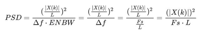
三步便完成了从fft到psd的转换。其中第一步和第二步和前面fft从two-sided转换到one-sided没有差别,重点就是第二步。在1中提到了FFT和PSD之间的关系:
其中S是第二节中用fft得到的amplitude spectrum,Δf 是 FFT 分辨率也就是 Fs/L,ENBW是噪声有效带宽,和FFT的窗函数有关。
以矩形为例,其ENBW=1,因此有
也就对应了Matlab官方链接中的
psdx = (1/(fs*N)) * abs(xdft).^2;
不过,公式是two-sided spectrum,乘以2即可转换到one-sided spectrum
【1】参考网址:https://www.ap.com/blog/fft-spectrum-and-spectral-densities-same-data-different-scaling
如何在 FFT 中观察到正弦信号的幅度
Fs = 1000; % Sampling frequency
T = 1/Fs; % Sampling period
L = 1500; % Length of signal
t = (0:L-1)*T; % Time vector
构造一个信号,其中包含振幅为 0.8 的 DC 偏移量、振幅为 0.7 的 50 Hz 正弦量和振幅为 1 的 120 Hz 正弦量。
S = 0.8 + 0.7*sin(2*pi*50*t) + sin(2*pi*120*t);
用均值为零、方差为 4 的随机噪声扰乱该信号。
X = S + 2*randn(size(t));
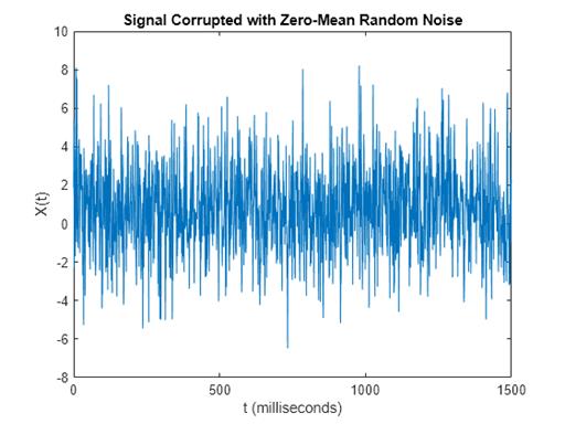
计算信号的傅里叶变换。
Y = fft(X);
由于傅里叶变换涉及复数,因此绘制 fft 频谱的复数模。
plot(Fs/L*(0:L-1),abs(Y),"LineWidth",3)
title("Complex Magnitude of fft Spectrum")
xlabel("f (Hz)")
ylabel("|fft(X)|")
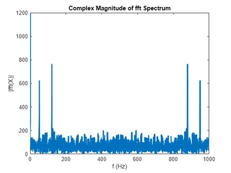
该图显示五个频率峰值,包括 DC 偏移量在 0 Hz 处的峰值。在此示例中,信号预计在 0 Hz、50 Hz 和 120 Hz 处有三个频率峰值。此处,绘图的后半部分是前半部分的镜像,不包括 0 Hz 处的峰值。原因是时域信号的离散傅里叶变换具有周期性,其频谱的前半部分为正频率,后半部分为负频率,第一个元素保留用于零频率。
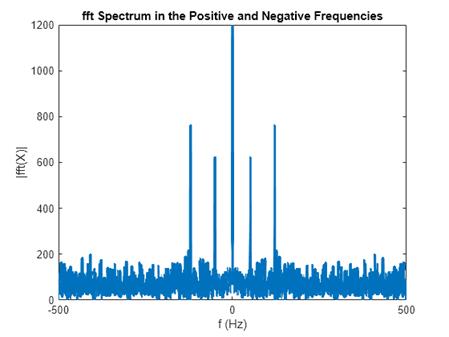
对于实信号,fft 频谱是双边频谱,其中正频率的频谱是负频率的频谱的复共轭。要显示正负频率的 fft 频谱,可以使用 fftshift。对于偶数长度 L,频域从奈奎斯特频率的负值 -Fs/2 开始,直到 Fs/2-Fs/L,间距或频率分辨率为 Fs/L。
plot(Fs/L*(-L/2:L/2-1),abs(fftshift(Y)),"LineWidth",3)
title("fft Spectrum in the Positive and Negative Frequencies")
xlabel("f (Hz)")
ylabel("|fft(X)|")
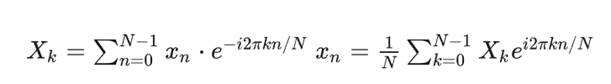
想在频谱上观察到sin信号的幅度,不能少的一件事是对fft结果除以L。观察IDFT的公式
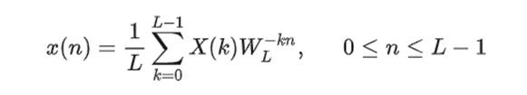
已经看到1/L了。IDFT公式其实也叫synthesis公式,它告诉我们拿到fft结果后(X(k),也就是Matlab的fft链接中的Y)如何还原原来的实数序列 x(n)。
这里可以看到:
为了找到三个频率峰值的幅值,将 Y 中的 fft 频谱转换为单边振幅频谱。由于 fft 函数包括原始信号和变换信号之间的缩放因子 L,因此通过除以 L 来重新缩放 Y。取 fft 频谱的复数模。双边振幅频谱 P2(其中正频率的频谱是负频率的频谱的复共轭),其峰值振幅是时域信号中对应峰值振幅的一半。要转换为单边频谱,取双边频谱 P2 的前半部分。将正频率的频谱乘以 2。您不需要将 P1(1) 和 P1(end) 乘以 2,因为这些振幅分别对应于零频率和奈奎斯特频率,并且在负频率下没有复共轭对组。
P2 = abs(Y/L);
P1 = P2(1:L/2+1);
P1(2:end-1) = 2*P1(2:end-1);
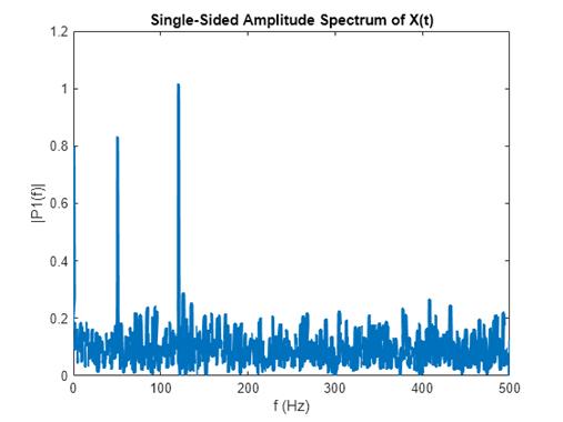
定义单边频谱的频域 f。绘制单边振幅频谱 P1。与预期相符,振幅接近 0.8、0.7 和 1,但由于增加了噪声,它们并不精确等于这些值。大多数情况下,较长的信号会产生更好的频率逼近值。
f = Fs/L*(0:(L/2));
plot(f,P1,"LineWidth",3)
title("Single-Sided Amplitude Spectrum of X(t)")
xlabel("f (Hz)")
ylabel("|P1(f)|")
参考文献
Heinzel, G., Rüdiger, A., & Schilling, R. (2002). 通过离散傅里叶变换(DFT)进行频谱和谱密度估计,包括一个全面的窗函数列表以及一些新的平顶窗。
- 参考网址:https://www.ap.com/blog/fft-spectrum-and-spectral-densities-same-data-different-scaling
- 参考网址:https://zhuanlan.zhihu.com/p/699960826
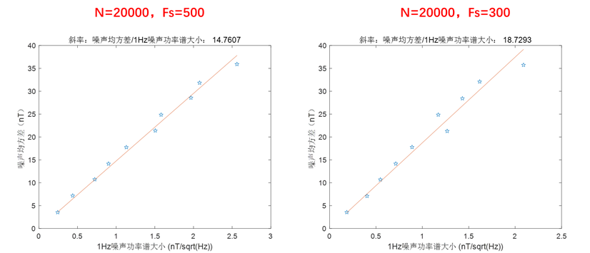
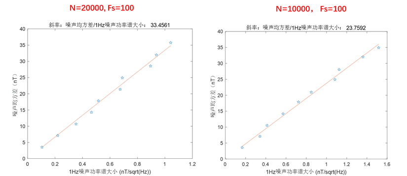
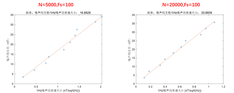
讨论方差与噪声功率谱的关系:
若FFT的公式是:matlab代码解释:
频域分析:从傅里叶变换到功率谱密度
一、 傅里叶变换
傅里叶变换是信号处理领域的基石,其精髓在于将时间域的信号转换到频域。在Matlab中,我们可以使用fft函数来进行傅里叶变换。
y = randn(1,1000); % 创建随机信号
Y = fft(y); % 傅里叶变换
傅里叶变换的结果是复数,包含了相位和幅度信息。在许多应用中,我们更关注信号在频率域上的能量分布,因此我们通常会计算其绝对值的平方,这也就引入了功率谱的概念。
二、功率谱
功率谱是信号在频率域上的能量分布。在Matlab中,我们可以基于傅里叶变换的结果计算功率谱:
Pxx = abs(Y).^2;
得到的Pxx就是我们的功率谱。然而,我们经常希望知道每一个频率单元的能量分布,这就引入了功率谱密度的概念。
三、功率谱密度
功率谱密度(PSD)是单位频率的能量分布。在Matlab中,我们可以通过除以频率分辨率来得到功率谱密度:
fs = 1000; % 采样频率
NFFT = length(y); % FFT的点数
f_res = fs / NFFT; % 频率分辨率
PSD = Pxx / f_res; % 功率谱密度,这里Pxx应该是归一化的
至此,我们介绍了三个基础概念:傅里叶变换、功率谱、功率谱密度。尽管这些概念彼此密切相关,但它们之间的区别也非常重要。
对于傅里叶变换、功率谱和功率谱密度的转换,关键在于明确频率的宽度。在傅里叶变换中,频率的宽度等于采样频率除以FFT点数。如果我们已经知道了功率谱,想要得到功率谱密度,就需要将功率谱除以频率的宽度;反过来,如果我们已经有了功率谱密度,想要得到功率谱,就需要将功率谱密度乘以频率的宽度。
然而,如果在进行FFT变换时,已经进行了标准化处理(即FFT的结果除以了样本长度),那么得到的实际上就是平均过的结果,也就是已经除以了频率的宽度。所以,在这种情况下,计算PSD时,我们只需要再除以采样率即可。因此,在这种情况下,功率谱可以直接由功率谱密度乘以采样率得出。
Y_norm = fft(y) / NFFT; % 标准化处理的FFT
Pxx_norm = abs(Y_norm).^2; % 标准化处理的功率谱
PSD_norm = Pxx_norm / fs; % 标准化处理的功率谱密度
% 这时,我们可以直接用PSD乘以fs来得到Pxx
Pxx_recovered = PSD_norm * fs;
附:幅值、功率、功率谱、功率谱密度计算代码
%做FFT变换,求真实幅值(uV)
temp = fft(y,NFFT)/ L;
Y(jj,:) = 2*abs(temp(1:NFFT/2+1));
% 做FFT变换,求功率(uV平方)
temp = 2 * abs(fft(y,NFFT)).^2/L;
Y(jj,:) = temp(1:NFFT/2+1);
% 做FFT变换,求功率谱密度(PSD)(单位 uV平方/Hz)
temp = 2*abs(fft(y,NFFT)).^2/L/Fs;
Y(jj,:) = temp(1:NFFT/2 + 1);
% 做FFT变换,求功率谱密度(PSD)(单位 dB )
temp = 2*abs(fft(y,NFFT)).^2/L/Fs;
Y(jj,:) = 10*log10(temp(1:NFFT/2+1));
总的来说,理解这些概念及其转换关系,是理解和分析信号的关键。尤其是在处理实际问题时,应当清楚的知道你的数据是功率谱还是功率谱密度,以便正确处理和解释结果。
FFT 归一化
一、背景
将时域信号转换为频域信号时,涉及到幅度和能量的变化,目前大部分开源库在正变换和反变换时会忽略常数,因此当我们想将频域和时域信号归一化到统一尺度时(方便设置阈值),需要做归一化操作。查找资料时发现有人使用1/N,2/N,有人说使用1/N, 其实这两种归一化都对,只是使用场景不同而已。
二、归一化方式
1 )单个频点幅度

2 )整帧能量
三、例子
clear
N = 2^8;
%data = randn(N,1);
f = 1000;
fs = 16000;
data = 3*sin(2*pi*f*(1:N)/fs) + 1;
%% 整帧归一化,关注整帧能量
dataFFT1 = fft(data)/sqrt(N);
powerError = (norm(data).^2 - norm(dataFFT1).^2);
%% 频点幅度归一化,关注单个频点幅度
dataFFT2 = 2 * fft(data)/N;
% dataFFT2 = dataFFT1 / sqrt(N) * 2;
dataFFT2(1,1) = dataFFT2(1,1) / 2;
dataAmp = sqrt(dataFFT2.*conj(dataFFT2));
figure
plot(dataAmp)
Matlab 利用离散傅里叶变换 DFT 进行频谱分析
参考网站:https://zhuanlan.zhihu.com/p/401208432
0. 原由
信号在频域能够呈现出时域不易发现的性质和规律,傅里叶变换是将信号从时域变换到频域,便于在频域对信号的特性进行分析。离散傅里叶变换 (DFT),是傅里叶变换在时域和频域上的离散呈现形式,通俗的说就是将经过采样的有限长度时域离散采样序列变换为等长度的频域离散采样序列,通过对变换得到的频域采样序列进行适当的换算和处理,可以得到信号的频谱(频率-幅值曲线和频率-相位曲线)。
1. 定义
离散傅里叶变换 (DFT)的定义为:
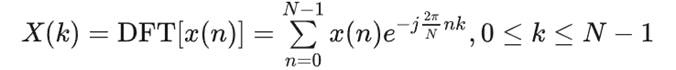
式中,x(n)为时域离散采样序列(通常为实数序列),N为时域离散采样序列x(n)的长度,X(k)为频域离散采样序列(通常为复数序列)。
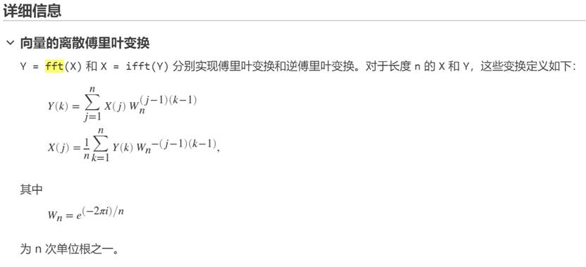
快速傅里叶变换(FFT)是离散傅里叶变换(DFT)的一种快速算法,FFT的计算结果与DFT完全相同,但FFT相对于DFT减小了计算量、节约计算资源消耗,能够适应在线计算,因此实际DFT都是通过FFT算法来求得结果。
Matlab软件自带fft函数实现快速傅里变换算法,但是光使用fft并不能直接得到信号的频谱,还需要解决以下问题:
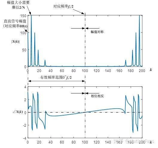
- 幅值变换:X(k)序列的幅值大小与参与变换的时域序列x(n)长度N有关,变换后的幅值|X(k)|需要乘以2/N得到真实幅值;
- 有效频率区域:X(k)序列由两部分共轭复数序列组成(复数共轭表示幅值相等、相位相反),相当于只有一半的复数序列是独立有效的,这部分复数序列对应0~fs/2的频率区域(fs为时域离散采样序列x(n)的采样频率)。
- 直流信号的处理:直流信号幅值(对应频率0Hz)为两部分共轭复数序列在频率0Hz处的加和,其真实幅值再乘以2/N后还需要再除以2得到真实的直流信号幅值。
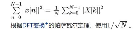
左边是PSD,归一化平方,右边是考虑信号幅度真实的FFT