Day 10 编程实战：Boosting（AdaBoost & GBDT）金融预测

Day 10 编程实战：Boosting（AdaBoost & GBDT）金融预测

实战目标

1. 理解 AdaBoost 和 GBDT 的核心原理
2. 使用 AdaBoostClassifier 进行涨跌预测
3. 使用 GradientBoostingClassifier 进行涨跌预测
4. 对比 Boosting 与随机森林的性能
5. 学习 GBDT 的超参数调优

1. 导入必要的库

import numpy as np
import pandas as pd
import matplotlib.pyplot as plt
import seaborn as sns
import time
from pathlib import Path
from sklearn.ensemble import (
    AdaBoostClassifier, GradientBoostingClassifier, 
    RandomForestClassifier
)
from sklearn.tree import DecisionTreeClassifier
from sklearn.model_selection import train_test_split, TimeSeriesSplit, GridSearchCV, cross_val_score
from sklearn.metrics import (
    accuracy_score, precision_score, recall_score, f1_score,
    roc_auc_score, roc_curve, classification_report, confusion_matrix
)
from sklearn.preprocessing import StandardScaler
import warnings
warnings.filterwarnings('ignore')

# 启用LaTeX渲染（如果系统安装了LaTeX）
plt.rcParams['text.usetex'] = False  # 设为False避免LaTeX依赖
# 设置中文显示
plt.rcParams['font.sans-serif'] = ['SimHei', 'Microsoft YaHei', 'DejaVu Sans']
plt.rcParams['axes.unicode_minus'] = False

2. 生成金融数据

def generate_financial_data(ts_code):
    """生成金融数据"""
    
    data_path = Path(r"E:\AppData\quant_trade\klines\kline2014-2024")
    kline_file = data_path / f"{ts_code}.csv"
    
    df = pd.read_csv(kline_file, usecols=["trade_date", "close", "vol"],
                     parse_dates=["trade_date"])\
            .rename(columns={"vol": "volume"})\
            .sort_values(by=["trade_date"])\
            .reset_index(drop=True)
    
    df['return'] = df['close'].pct_change()
    
    # 技术指标
    # RSI
    delta = df['return'].fillna(0)
    gain = delta.where(delta > 0, 0).rolling(14).mean()
    loss = -delta.where(delta < 0, 0).rolling(14).mean()
    rs = gain / (loss + 1e-10)
    df['rsi'] = 100 - (100 / (1 + rs))
    
    # MACD
    ema12 = df['close'].ewm(span=12, adjust=False).mean()
    ema26 = df['close'].ewm(span=26, adjust=False).mean()
    df['macd'] = ema12 - ema26
    df['macd_signal'] = df['macd'].ewm(span=9, adjust=False).mean()
    
    # 均线比率
    df['ma5'] = df['close'].rolling(5).mean()
    df['ma20'] = df['close'].rolling(20).mean()
    df['ma_ratio'] = df['ma5'] / df['ma20'] - 1
    
    # 波动率
    df['volatility'] = df['return'].rolling(20).std()
    
    # 成交量比率
    df['volume_ratio'] = df['volume'] / df['volume'].rolling(10).mean()
    
    # 动量指标
    for lag in [1, 2, 3, 5, 10]:
        df[f'momentum_{lag}'] = df['return'].shift(lag).fillna(0)
    
    # 目标变量：次日是否上涨
    df['target'] = (df['return'].shift(-1) > 0).astype(int)
    
    # 删除缺失值
    df = df.dropna()
    
    return df

# 生成数据
ts_code = '600519.SH'
df = generate_financial_data(ts_code)
print(f"数据形状: {df.shape}")

# 特征选择
feature_cols = ['rsi', 'macd', 'macd_signal', 'ma_ratio', 'volatility', 
                'volume_ratio', 'momentum_1', 'momentum_2', 'momentum_3', 
                'momentum_5', 'momentum_10']
X = df[feature_cols]
y = df['target']

print(f"特征数量: {len(feature_cols)}")
print(f"样本数量: {len(X)}")
print(f"目标分布: \n{y.value_counts(normalize=True)}")

# 按时间划分
split_idx = int(len(X) * 0.7)
X_train = X[:split_idx]
X_test = X[split_idx:]
y_train = y[:split_idx]
y_test = y[split_idx:]

print(f"\n训练集: {len(X_train)} 样本")
print(f"测试集: {len(X_test)} 样本")

数据形状: (2452, 18)
特征数量: 11
样本数量: 2452
目标分布: 
target
1    0.505302
0    0.494698
Name: proportion, dtype: float64

训练集: 1716 样本
测试集: 736 样本

3. AdaBoost 算法详解与实现

3.1 手动实现 AdaBoost

class AdaBoostManual:
    """手动实现 AdaBoost（演示原理）"""
    
    def __init__(self, n_estimators=50, learning_rate=1.0):
        self.n_estimators = n_estimators
        self.learning_rate = learning_rate
        self.models = []
        self.model_weights = []
    
    def fit(self, X, y):
        """
        这里标签 y 是 -1 和 +1
        """
        n_samples = len(X)
        # 初始化样本权重
        weights = np.ones(n_samples) / n_samples
        
        for t in range(self.n_estimators):
            # 训练弱学习器（决策树桩）
            stump = DecisionTreeClassifier(max_depth=1, random_state=t)
            stump.fit(X, y, sample_weight=weights)
            
            # 预测
            y_pred = stump.predict(X)
            
            # 计算加权误差率
            error = np.sum(weights * (y_pred != y)) / np.sum(weights)
            
            # 计算模型权重
            alpha = 0.5 * np.log((1 - error) / (error + 1e-10))
            alpha = alpha * self.learning_rate
            
            # 更新样本权重
            ## sklearn 的决策树输出通常是 0 和 1。
            ## AdaBoost 的数学公式要求标签是 -1 和 +1。
            ## 这行代码把预测结果从 [0, 1] 映射到了 [-1, +1]。
            weights = weights * np.exp(-alpha * y * (2 * y_pred - 1))
            weights = weights / np.sum(weights)  # 归一化
            
            # 保存模型
            self.models.append(stump)
            self.model_weights.append(alpha)
            
            # 打印进度
            if (t + 1) % 10 == 0:
                print(f"迭代 {t+1}/{self.n_estimators}, 误差率: {error:.4f}, α: {alpha:.4f}")
        
        return self
    
    def predict(self, X):
        # 加权投票
        pred_sum = np.zeros(len(X))
        for alpha, model in zip(self.model_weights, self.models):
            pred_sum += alpha * (2 * model.predict(X) - 1)
        return (pred_sum > 0).astype(int)

# 测试手动实现
print("="*60)
print("手动实现 AdaBoost 测试")
print("="*60)
X_sample = X_train[:1000]
y_sample = y_train[:1000]

ada_manual = AdaBoostManual(n_estimators=30)
ada_manual.fit(X_sample, 2 * y_sample -1)
y_pred_manual = ada_manual.predict(X_test)

print(f"\n手动实现 AdaBoost 测试集准确率: {accuracy_score(y_test, y_pred_manual):.4f}")

============================================================
手动实现 AdaBoost 测试
============================================================
迭代 10/30, 误差率: 0.4233, α: 0.1546
迭代 20/30, 误差率: 0.4693, α: 0.0614
迭代 30/30, 误差率: 0.4921, α: 0.0158

手动实现 AdaBoost 测试集准确率: 0.4810

3.2 使用 sklearn 的 AdaBoost

print("="*60)
print("sklearn AdaBoost 训练")
print("="*60)

# 基础 AdaBoost（决策树桩）
ada_base = AdaBoostClassifier(
    n_estimators=100,
    learning_rate=1.0,
    random_state=42
)

start_time = time.time()
ada_base.fit(X_train, y_train)
ada_time = time.time() - start_time

# 预测
y_pred_ada = ada_base.predict(X_test)
y_proba_ada = ada_base.predict_proba(X_test)[:, 1]

print(f"训练时间: {ada_time:.2f}秒")
print(f"测试集准确率: {accuracy_score(y_test, y_pred_ada):.4f}")
print(f"AUC: {roc_auc_score(y_test, y_proba_ada):.4f}")

# 不同基学习器
print("\n使用浅层决策树作为基学习器:")
ada_tree = AdaBoostClassifier(
    estimator=DecisionTreeClassifier(max_depth=3),
    n_estimators=100,
    learning_rate=0.5,
    random_state=42
)
ada_tree.fit(X_train, y_train)
y_pred_ada_tree = ada_tree.predict(X_test)
y_proba_ada_tree = ada_tree.predict_proba(X_test)[:, 1]

print(f"测试集准确率: {accuracy_score(y_test, y_pred_ada_tree):.4f}")
print(f"AUC: {roc_auc_score(y_test, y_proba_ada_tree):.4f}")

============================================================
sklearn AdaBoost 训练
============================================================
训练时间: 0.59秒
测试集准确率: 0.5027
AUC: 0.5114

使用浅层决策树作为基学习器:
测试集准确率: 0.4986
AUC: 0.5039

3.3 AdaBoost 参数影响分析

def analyze_adaboost_params(X_train, y_train, X_test, y_test):
    """分析 AdaBoost 的 n_estimators 和 learning_rate 影响"""
    
    n_range = [10, 20, 50, 100, 200, 300]
    lr_range = [0.1, 0.5, 1.0, 1.5, 2.0]
    
    results = []
    
    for n in n_range:
        for lr in lr_range:
            ada = AdaBoostClassifier(n_estimators=n, learning_rate=lr, random_state=42)
            ada.fit(X_train, y_train)
            y_pred = ada.predict(X_test)
            acc = accuracy_score(y_test, y_pred)
            results.append({'n_estimators': n, 'learning_rate': lr, 'accuracy': acc})
    
    results_df = pd.DataFrame(results)
    
    # 创建热力图
    pivot_table = results_df.pivot(index='n_estimators', columns='learning_rate', values='accuracy')
    
    plt.figure(figsize=(10, 6))
    sns.heatmap(pivot_table, annot=True, fmt='.4f', cmap='RdYlGn', center=0.5)
    plt.title('AdaBoost 参数热力图（测试集准确率）')
    plt.xlabel('学习率 (learning_rate)')
    plt.ylabel('树数量 (n_estimators)')
    plt.tight_layout()
    plt.show()
    
    # 最佳参数
    best_row = results_df.loc[results_df['accuracy'].idxmax()]
    print(f"最佳参数: n_estimators={int(best_row['n_estimators'])}, learning_rate={best_row['learning_rate']}")
    print(f"最佳准确率: {best_row['accuracy']:.4f}")
    
    return best_row

# 分析 AdaBoost 参数（使用子集加速）
print("分析 AdaBoost 参数影响...")
X_sample = X_train[:2000]
y_sample = y_train[:2000]
best_ada_params = analyze_adaboost_params(X_sample, y_sample, X_test, y_test)

分析 AdaBoost 参数影响...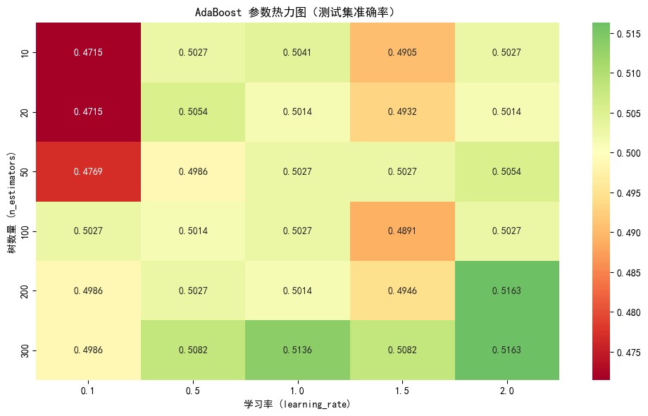

最佳参数: n_estimators=200, learning_rate=2.0
最佳准确率: 0.5163

4. GBDT 算法详解与实现

4.1 梯度提升分类器基础

print("="*60)
print("GradientBoostingClassifier 训练")
print("="*60)

# 基础 GBDT
gbdt_base = GradientBoostingClassifier(
    n_estimators=100,
    learning_rate=0.1,
    max_depth=3,
    random_state=42
)

start_time = time.time()
gbdt_base.fit(X_train, y_train)
gbdt_time = time.time() - start_time

# 预测
y_pred_gbdt = gbdt_base.predict(X_test)
y_proba_gbdt = gbdt_base.predict_proba(X_test)[:, 1]

print(f"训练时间: {gbdt_time:.2f}秒")
print(f"测试集准确率: {accuracy_score(y_test, y_pred_gbdt):.4f}")
print(f"精确率: {precision_score(y_test, y_pred_gbdt):.4f}")
print(f"召回率: {recall_score(y_test, y_pred_gbdt):.4f}")
print(f"F1: {f1_score(y_test, y_pred_gbdt):.4f}")
print(f"AUC: {roc_auc_score(y_test, y_proba_gbdt):.4f}")

# 特征重要性
feature_importance_gbdt = pd.DataFrame({
    'feature': feature_cols,
    'importance': gbdt_base.feature_importances_
}).sort_values('importance', ascending=False)

print("\n特征重要性（Top 5）:")
print(feature_importance_gbdt.head())

============================================================
GradientBoostingClassifier 训练
============================================================
训练时间: 1.06秒
测试集准确率: 0.4918
精确率: 0.4737
召回率: 0.7003
F1: 0.5651
AUC: 0.5038

特征重要性（Top 5）:
         feature  importance
8     momentum_3    0.130215
5   volume_ratio    0.116798
7     momentum_2    0.104701
4     volatility    0.104672
10   momentum_10    0.103805

4.2 不同损失函数对比

def compare_gbdt_loss_functions(X_train, y_train, X_test, y_test):
    """对比不同损失函数的性能"""

    # 旧版本损失函数 deviance 改为 log_loss，
    loss_functions = ['log_loss', 'exponential']
    results = []
    
    for loss in loss_functions:
        gbdt = GradientBoostingClassifier(
            n_estimators=100,
            learning_rate=0.1,
            max_depth=3,
            loss=loss,
            random_state=42
        )
        gbdt.fit(X_train, y_train)
        
        y_pred = gbdt.predict(X_test)
        y_proba = gbdt.predict_proba(X_test)[:, 1]
        
        results.append({
            'loss': loss,
            'accuracy': accuracy_score(y_test, y_pred),
            'precision': precision_score(y_test, y_pred),
            'recall': recall_score(y_test, y_pred),
            'f1': f1_score(y_test, y_pred),
            'auc': roc_auc_score(y_test, y_proba)
        })
    
    results_df = pd.DataFrame(results)
    print("\n不同损失函数性能对比:")
    print(results_df.to_string(index=False))
    
    return results_df

compare_gbdt_loss_functions(X_train, y_train, X_test, y_test)

不同损失函数性能对比:
       loss  accuracy  precision   recall       f1      auc
   log_loss  0.491848   0.473684 0.700288 0.565116 0.503812
exponential  0.480978   0.464066 0.651297 0.541966 0.496440

4.3 学习率与树数量的关系

def analyze_lr_vs_trees(X_train, y_train, X_test, y_test):
    """分析学习率和树数量的关系"""
    
    learning_rates = [0.01, 0.05, 0.1, 0.2, 0.3]
    n_estimators_list = [50, 100, 200, 300]
    
    results = []
    
    for lr in learning_rates:
        for n in n_estimators_list:
            gbdt = GradientBoostingClassifier(
                n_estimators=n,
                learning_rate=lr,
                max_depth=3,
                random_state=42
            )
            gbdt.fit(X_train, y_train)
            y_proba = gbdt.predict_proba(X_test)[:, 1]
            auc = roc_auc_score(y_test, y_proba)
            results.append({
                'learning_rate': lr,
                'n_estimators': n,
                'auc': auc
            })
    
    results_df = pd.DataFrame(results)
    
    # 绘图
    plt.figure(figsize=(10, 6))
    for lr in learning_rates:
        subset = results_df[results_df['learning_rate'] == lr]
        plt.plot(subset['n_estimators'], subset['auc'], 'o-', label=f'lr={lr}', linewidth=2)
    
    plt.xlabel('树数量 (n_estimators)')
    plt.ylabel('AUC')
    plt.title('学习率与树数量对GBDT性能的影响')
    plt.legend()
    plt.grid(True, alpha=0.3)
    plt.show()
    
    # 最佳组合
    best = results_df.loc[results_df['auc'].idxmax()]
    print(f"最佳组合: learning_rate={best['learning_rate']}, n_estimators={best['n_estimators']}")
    print(f"最佳AUC: {best['auc']:.4f}")
    
    return best

analyze_lr_vs_trees(X_train, y_train, X_test, y_test)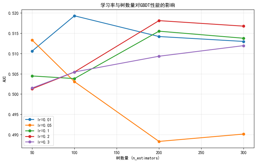

最佳组合: learning_rate=0.01, n_estimators=100.0
最佳AUC: 0.5193
learning_rate      0.010000
n_estimators     100.000000
auc                0.519302
Name: 1, dtype: float64

5. GBDT 超参数调优

5.1 网格搜索

def grid_search_gbdt(X_train, y_train, X_test, y_test):
    """GBDT 网格搜索"""
    
    # 定义参数网格
    param_grid = {
        'n_estimators': [100, 200],
        'max_depth': [3, 4, 5],
        'min_samples_split': [2, 5, 10],
        'learning_rate': [0.05, 0.1]
    }
    
    # 时间序列交叉验证
    tscv = TimeSeriesSplit(n_splits=3)
    
    gbdt = GradientBoostingClassifier(random_state=42)
    
    grid_search = GridSearchCV(
        gbdt, param_grid,
        cv=tscv,
        scoring='roc_auc',
        n_jobs=-1,
        verbose=1
    )
    
    print("开始网格搜索...")
    start_time = time.time()
    grid_search.fit(X_train, y_train)
    elapsed = time.time() - start_time
    
    print(f"\n搜索完成，耗时: {elapsed:.2f}秒")
    print(f"最佳参数: {grid_search.best_params_}")
    print(f"最佳CV AUC: {grid_search.best_score_:.4f}")
    
    # 测试集评估
    y_pred = grid_search.predict(X_test)
    y_proba = grid_search.predict_proba(X_test)[:, 1]
    
    print(f"\n测试集准确率: {accuracy_score(y_test, y_pred):.4f}")
    print(f"测试集AUC: {roc_auc_score(y_test, y_proba):.4f}")
    
    return grid_search.best_estimator_

# 执行网格搜索（使用子集加速）
print("GBDT 超参数调优...")
X_sample = X_train[:2000]
y_sample = y_train[:2000]
best_gbdt = grid_search_gbdt(X_sample, y_sample, X_test, y_test)

GBDT 超参数调优...
开始网格搜索...
Fitting 3 folds for each of 36 candidates, totalling 108 fits

搜索完成，耗时: 38.98秒
最佳参数: {'learning_rate': 0.05, 'max_depth': 5, 'min_samples_split': 10, 'n_estimators': 200}
最佳CV AUC: 0.5195

测试集准确率: 0.4918
测试集AUC: 0.5108

5.2 早停（Early Stopping）

def early_stopping_demo(X_train, y_train, X_test, y_test):
    """演示早停机制"""
    
    # 划分验证集
    split_idx = int(len(X_train) * 0.8)
    X_train_sub = X_train[:split_idx]
    y_train_sub = y_train[:split_idx]
    X_val = X_train[split_idx:]
    y_val = y_train[split_idx:]
    
    # 训练不同树数量的模型
    n_estimators_list = range(10, 310, 20)
    train_scores = []
    val_scores = []
    
    for n in n_estimators_list:
        gbdt = GradientBoostingClassifier(
            n_estimators=n,
            learning_rate=0.1,
            max_depth=3,
            random_state=42
        )
        gbdt.fit(X_train_sub, y_train_sub)
        
        train_scores.append(roc_auc_score(y_train_sub, gbdt.predict_proba(X_train_sub)[:, 1]))
        val_scores.append(roc_auc_score(y_val, gbdt.predict_proba(X_val)[:, 1]))
    
    # 绘图
    plt.figure(figsize=(10, 6))
    plt.plot(n_estimators_list, train_scores, 'b-o', label='训练集', linewidth=2)
    plt.plot(n_estimators_list, val_scores, 'r-s', label='验证集', linewidth=2)
    plt.xlabel('树数量 (n_estimators)')
    plt.ylabel('AUC')
    plt.title('早停原理：验证集AUC先升后降')
    plt.legend()
    plt.grid(True, alpha=0.3)
    
    # 标记最佳点
    best_idx = np.argmax(val_scores)
    best_n = n_estimators_list[best_idx]
    plt.axvline(x=best_n, color='green', linestyle='--', label=f'最佳树数量={best_n}')
    plt.legend()
    plt.show()
    
    print(f"最佳树数量: {best_n}")
    print(f"训练集AUC: {train_scores[best_idx]:.4f}")
    print(f"验证集AUC: {val_scores[best_idx]:.4f}")

early_stopping_demo(X_train, y_train, X_test, y_test)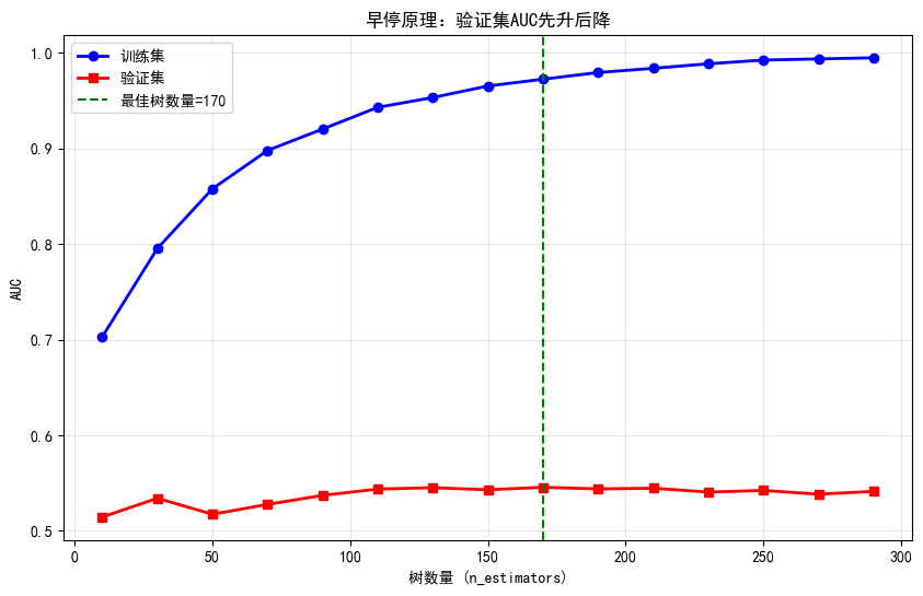

最佳树数量: 170
训练集AUC: 0.9723
验证集AUC: 0.5456

6. 模型综合对比

6.1 训练所有模型

print("="*70)
print("模型综合对比")
print("="*70)

# 随机森林
rf = RandomForestClassifier(n_estimators=100, max_depth=10, random_state=42, n_jobs=-1)
rf.fit(X_train, y_train)
rf_pred = rf.predict(X_test)
rf_proba = rf.predict_proba(X_test)[:, 1]

# AdaBoost
ada = AdaBoostClassifier(n_estimators=100, learning_rate=1.0, random_state=42)
ada.fit(X_train, y_train)
ada_pred = ada.predict(X_test)
ada_proba = ada.predict_proba(X_test)[:, 1]

# GBDT
gbdt = GradientBoostingClassifier(n_estimators=100, learning_rate=0.1, max_depth=3, random_state=42)
gbdt.fit(X_train, y_train)
gbdt_pred = gbdt.predict(X_test)
gbdt_proba = gbdt.predict_proba(X_test)[:, 1]

# 收集结果
models = {
    '随机森林': (rf_pred, rf_proba),
    'AdaBoost': (ada_pred, ada_proba),
    'GBDT': (gbdt_pred, gbdt_proba)
}

results = []
for name, (pred, proba) in models.items():
    results.append({
        '模型': name,
        '准确率': accuracy_score(y_test, pred),
        '精确率': precision_score(y_test, pred),
        '召回率': recall_score(y_test, pred),
        'F1': f1_score(y_test, pred),
        'AUC': roc_auc_score(y_test, proba)
    })

results_df = pd.DataFrame(results)
print("\n性能对比:")
print(results_df.to_string(index=False))

======================================================================
模型综合对比
======================================================================

性能对比:
      模型      准确率      精确率      召回率       F1      AUC
    随机森林 0.502717 0.481973 0.731988 0.581236 0.500100
AdaBoost 0.502717 0.483536 0.804035 0.603896 0.511353
    GBDT 0.491848 0.473684 0.700288 0.565116 0.503812

6.2 ROC曲线对比

plt.figure(figsize=(12, 8))

colors = {'随机森林': 'blue', 'AdaBoost': 'green', 'GBDT': 'red'}
for name, (_, proba) in models.items():
    fpr, tpr, _ = roc_curve(y_test, proba)
    auc = roc_auc_score(y_test, proba)
    plt.plot(fpr, tpr, color=colors[name], linewidth=2, 
             label=f'{name} (AUC={auc:.4f})')

plt.plot([0, 1], [0, 1], 'k--', linewidth=1, label='随机分类器')
plt.xlabel('假阳性率 (FPR)')
plt.ylabel('真阳性率 (TPR)')
plt.title('Boosting vs 随机森林 ROC曲线对比')
plt.legend(loc='lower right')
plt.grid(True, alpha=0.3)
plt.show()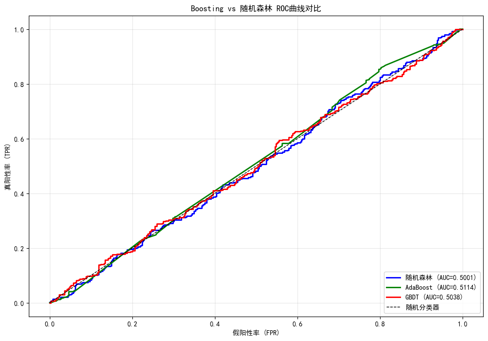

6.3 混淆矩阵对比

fig, axes = plt.subplots(1, 3, figsize=(15, 4))

for idx, (name, (pred, _)) in enumerate(models.items()):
    cm = confusion_matrix(y_test, pred)
    sns.heatmap(cm, annot=True, fmt='d', cmap='Blues', ax=axes[idx],
                xticklabels=['下跌', '上涨'], yticklabels=['下跌', '上涨'])
    axes[idx].set_title(f'{name}\n准确率: {accuracy_score(y_test, pred):.4f}')
    axes[idx].set_xlabel('预测')
    axes[idx].set_ylabel('真实')

plt.tight_layout()
plt.show()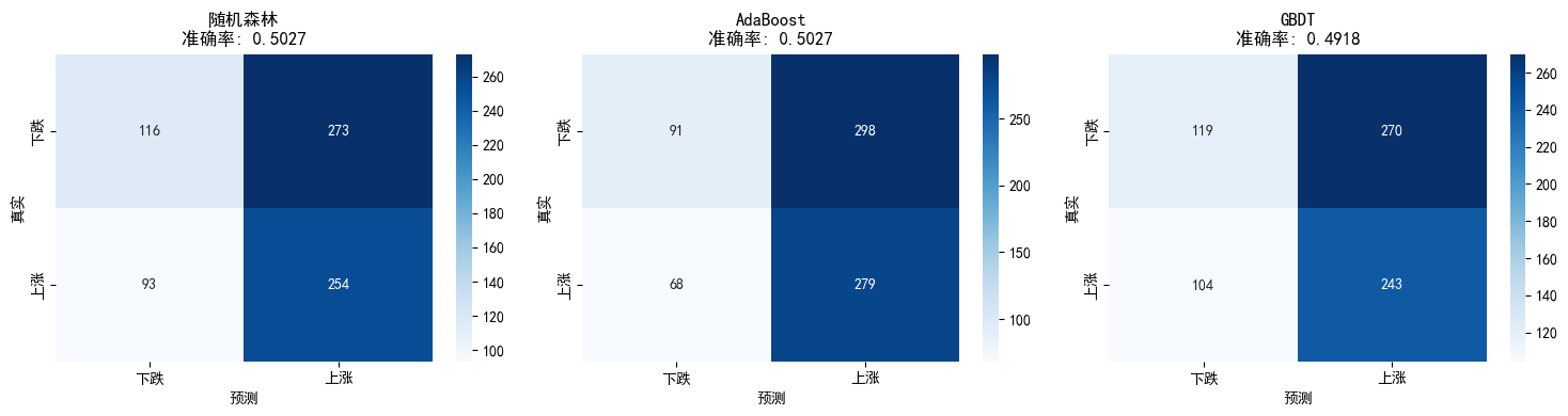

7. GBDT 特征重要性分析

7.1 特征重要性可视化

# 获取特征重要性
importances_gbdt = gbdt.feature_importances_
importance_df = pd.DataFrame({
    'feature': feature_cols,
    'importance': importances_gbdt
}).sort_values('importance', ascending=True)

plt.figure(figsize=(10, 6))
plt.barh(importance_df['feature'], importance_df['importance'])
plt.xlabel('重要性')
plt.title('GBDT 特征重要性')
for i, (_, row) in enumerate(importance_df.iterrows()):
    plt.text(row['importance'] + 0.002, i, f"{row['importance']:.4f}", va='center')
plt.grid(True, alpha=0.3)
plt.tight_layout()
plt.show()

print("特征重要性排序:")
print(importance_df.sort_values('importance', ascending=False).to_string(index=False))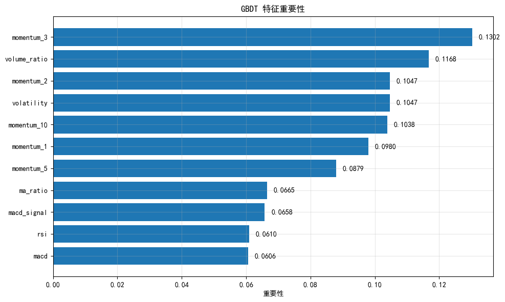

特征重要性排序:
     feature  importance
  momentum_3    0.130215
volume_ratio    0.116798
  momentum_2    0.104701
  volatility    0.104672
 momentum_10    0.103805
  momentum_1    0.097966
  momentum_5    0.087941
    ma_ratio    0.066498
 macd_signal    0.065796
         rsi    0.061013
        macd    0.060596

7.2 累积重要性曲线

# 累积重要性
sorted_importance = importance_df.sort_values('importance', ascending=False)['importance'].values
cumulative_importance = np.cumsum(sorted_importance)

plt.figure(figsize=(10, 6))
plt.plot(range(1, len(cumulative_importance) + 1), cumulative_importance, 'bo-', linewidth=2)
plt.axhline(y=0.9, color='r', linestyle='--', label='90% 阈值')
plt.axhline(y=0.95, color='g', linestyle='--', label='95% 阈值')
plt.xlabel('特征数量')
plt.ylabel('累积重要性')
plt.title('GBDT 累积特征重要性')
plt.legend()
plt.grid(True, alpha=0.3)

# 找到达到90%的特征数量
n_90 = np.argmax(cumulative_importance >= 0.9) + 1
n_95 = np.argmax(cumulative_importance >= 0.95) + 1
plt.axvline(x=n_90, color='r', linestyle=':', alpha=0.5)
plt.axvline(x=n_95, color='g', linestyle=':', alpha=0.5)
plt.text(n_90, 0.5, f'{n_90}个特征达90%', rotation=90)
plt.text(n_95, 0.5, f'{n_95}个特征达95%', rotation=90)

plt.show()

print(f"前 {n_90} 个特征贡献了 90% 的重要性")
print(f"前 {n_95} 个特征贡献了 95% 的重要性")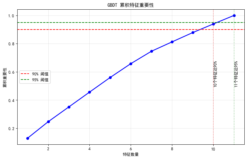

前 10 个特征贡献了 90% 的重要性
前 11 个特征贡献了 95% 的重要性

8. 学习曲线分析

GBDT 学习曲线

def plot_gbdt_learning_curve(X_train, y_train, X_val, y_val, max_estimators=300):
    """绘制GBDT的学习曲线"""
    
    train_scores = []
    val_scores = []
    n_list = range(10, max_estimators + 10, 20)
    
    for n in n_list:
        gbdt = GradientBoostingClassifier(
            n_estimators=n,
            learning_rate=0.1,
            max_depth=3,
            random_state=42
        )
        gbdt.fit(X_train, y_train)
        
        train_scores.append(roc_auc_score(y_train, gbdt.predict_proba(X_train)[:, 1]))
        val_scores.append(roc_auc_score(y_val, gbdt.predict_proba(X_val)[:, 1]))
    
    plt.figure(figsize=(10, 6))
    plt.plot(n_list, train_scores, 'b-o', label='训练集', linewidth=2)
    plt.plot(n_list, val_scores, 'r-s', label='验证集', linewidth=2)
    plt.xlabel('树数量 (n_estimators)')
    plt.ylabel('AUC')
    plt.title('GBDT 学习曲线')
    plt.legend()
    plt.grid(True, alpha=0.3)
    
    # 标记最佳点
    best_idx = np.argmax(val_scores)
    best_n = n_list[best_idx]
    plt.axvline(x=best_n, color='green', linestyle='--', label=f'最佳={best_n}')
    plt.legend()
    plt.show()
    
    print(f"最佳树数量: {best_n}")
    print(f"训练集AUC: {train_scores[best_idx]:.4f}")
    print(f"验证集AUC: {val_scores[best_idx]:.4f}")
    print(f"过拟合差距: {train_scores[best_idx] - val_scores[best_idx]:.4f}")

# 划分验证集
split_val = int(len(X_train) * 0.8)
X_train_sub = X_train[:split_val]
y_train_sub = y_train[:split_val]
X_val = X_train[split_val:]
y_val = y_train[split_val:]

plot_gbdt_learning_curve(X_train_sub, y_train_sub, X_val, y_val)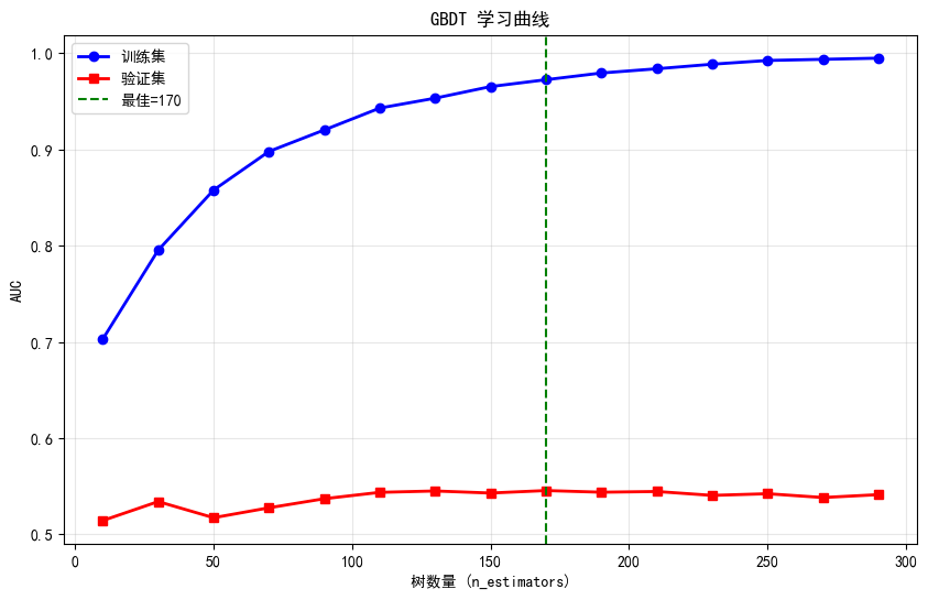

最佳树数量: 170
训练集AUC: 0.9723
验证集AUC: 0.5456
过拟合差距: 0.4266

9. Boosting vs Bagging 深入对比

偏差-方差分解

def bias_variance_analysis(X_train, y_train, X_test, y_test, n_experiments=10):
    """分析模型的偏差和方差"""
    
    models = {
        '随机森林': RandomForestClassifier(n_estimators=100, max_depth=10, random_state=None),
        'GBDT': GradientBoostingClassifier(n_estimators=100, learning_rate=0.1, max_depth=3, random_state=None)
    }
    
    results = {}
    
    for name, model in models.items():
        predictions = []
        
        for seed in range(n_experiments):
            np.random.seed(seed)
            model.set_params(random_state=seed)
            
            # 使用不同的训练子集
            indices = np.random.choice(len(X_train), len(X_train), replace=True)
            X_sample = X_train.iloc[indices]
            y_sample = y_train.iloc[indices]
            
            model.fit(X_sample, y_sample)
            pred = model.predict(X_test)
            predictions.append(pred)
        
        predictions = np.array(predictions)
        
        # 计算偏差和方差
        mean_pred = np.mean(predictions, axis=0)
        bias = np.mean(mean_pred != y_test)
        variance = np.mean(np.var(predictions, axis=0))
        
        results[name] = {'bias': bias, 'variance': variance}
    
    return pd.DataFrame(results).T

# 偏差-方差分析（使用子集加速）
print("偏差-方差分析（10次实验）...")
X_sample_analysis = X_train[:1000]
y_sample_analysis = y_train[:1000]
bias_var_df = bias_variance_analysis(X_sample_analysis, y_sample_analysis, X_test, y_test)

print("\n偏差-方差分析结果:")
print(bias_var_df)

# 可视化
fig, axes = plt.subplots(1, 2, figsize=(12, 5))

axes[0].bar(bias_var_df.index, bias_var_df['bias'])
axes[0].set_ylabel('偏差')
axes[0].set_title('模型偏差对比（越低越好）')
axes[0].grid(True, alpha=0.3)

axes[1].bar(bias_var_df.index, bias_var_df['variance'])
axes[1].set_ylabel('方差')
axes[1].set_title('模型方差对比（越低越好）')
axes[1].grid(True, alpha=0.3)

plt.tight_layout()
plt.show()

print("\n解读:")
print("- 随机森林: 方差较低（Bagging优势），偏差可能略高")
print("- GBDT: 偏差较低（Boosting优势），方差可能较高")
print("- 理想模型: 低偏差 + 低方差（需要平衡）")

偏差-方差分析（10次实验）...

偏差-方差分析结果:
          bias  variance
随机森林  0.877717  0.137622
GBDT  0.938859  0.170421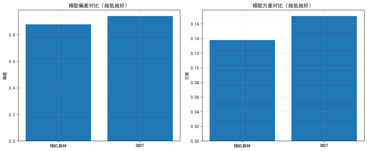

​

解读:
- 随机森林: 方差较低（Bagging优势），偏差可能略高
- GBDT: 偏差较低（Boosting优势），方差可能较高
- 理想模型: 低偏差 + 低方差（需要平衡）

10. 今日总结

================================================================================
                        Day 10 学习总结
================================================================================

1. Boosting 核心概念：

   • 串行训练，关注错误样本
   • 加权组合弱学习器
   • 降低偏差，可能增加方差

2. AdaBoost：

   • 调整样本权重和模型权重
   • 指数损失函数
   • 对异常值敏感

3. GBDT：

   • 函数空间梯度下降
   • 拟合负梯度（伪残差）
   • 支持多种损失函数

4. 超参数要点：

   • learning_rate × n_estimators ≈ 常数
   • 小学习率 + 多棵树通常更好
   • 使用早停防止过拟合

5. 模型对比：

   • 随机森林: 方差低，对异常值鲁棒
   • AdaBoost: 简单高效，但敏感
   • GBDT: 精度高，需要调参

6. 量化应用建议：

   • 先用随机森林作为基准
   • 如需更高精度，尝试GBDT
   • 注意防止时间序列过拟合
   • 使用时间序列交叉验证

7. 扩展作业

   • 作业1：实现自定义的GBDT损失函数
   • 作业2：使用早停训练GBDT，找到最佳树数量
   • 作业3：在实际股票数据上对比AdaBoost、GBDT和XGBoost
   • 作业4：分析GBDT的预测概率是否校准（使用校准曲线）

8. 量化思考

   • Boosting模型通常比随机森林精度更高
   • 但更容易过拟合，需要更谨慎的验证
   • 学习率是关键参数，建议从0.05开始
   • 时间序列数据建议使用TimeSeriesSplit验证