06-多头注意力机制 🎯
本文档深入讲解多头注意力机制(Multi-Head Attention)的核心原理,涵盖多头注意力的概念定义与设计动机、数学公式的完整推导、手动代码实现及逐行解析、PyTorch 原生 nn.MultiheadAttention 的使用方法、多头注意力权重的可视化对比,以及一个完整可运行的综合示例。通过理论与实践相结合的方式,帮助读者彻底吃透多头注意力机制 🛠️
📖 前置阅读 :本文档是 05-自注意力机制详解(CSDN)的进阶篇,建议先掌握自注意力机制再学习本文。代码实现部分可配合 04-缩放点积注意力代码实现(CSDN)一起阅读。
章节阅读路线图 🗺️
阅读顺序说明:
- 第1章 → 第2章:先建立多头注意力的概念认知,再深入数学原理
- 第2章 → 第3章:理解公式后,动手写代码实现
- 第3章 → 第4章:掌握手动实现后,学习 PyTorch 提供的优化版本
- 第4章 → 第5章:有了代码基础,可视化不同注意力头的权重分布
- 第5章 → 第6章:把所有内容整合成一个完整可运行的示例
1. 什么是多头注意力机制 🤔
本章介绍多头注意力的核心定义、设计动机及其与单头注意力的本质区别
1.1 核心定义 📝
多头注意力机制(Multi-Head Attention)是 Transformer 架构的核心创新之一。它不再只做一次注意力计算,而是将 Q、K、V 分别通过 h 组不同的线性投影,并行执行 h 次缩放点积注意力,最后将 h 个头的输出拼接起来再做一次线性变换。
用一句话概括:多头注意力 = 多个注意力头并行计算 + 结果拼接融合。
scss
MultiHead(Q, K, V) = Concat(head_1, head_2, ..., head_h) × W^O

其中每个头:
head_i = Attention(Q × W_i^Q, K × W_i^K, V × W_i^V)
参考资料:
- Attention Is All You Need -- arXiv ⭐值得阅读
- The Illustrated Transformer -- Jay Alammar ⭐值得阅读
- Multi-Head Attention Explained -- DigitalOcean
1.2 为什么需要多个头?------设计动机 🎯
单头注意力只在一个表示子空间中计算注意力,这意味着模型只能学到一种"关注模式"。但语言是极其复杂的------同一个词在不同语境下,可能需要关注:
- 语法关系:主语-谓语搭配、形容词-名词修饰
- 语义关系:同义词、反义词、上下位词
- 长距离依赖:代词指代、跨句关联
- 局部模式:相邻词的短语结构
单头注意力在训练过程中会收敛到单一最优解 ,倾向于优先关注最显著的关系模式(如语法关系或局部依赖),而无法灵活适应不同语境下的多样化需求 。单头注意力无法同时捕捉这些不同层面的关系。多头注意力的核心思想是:让不同的头关注不同的"表示子空间",每个头专攻一种关系模式。
直观类比:想象一个新闻编辑室------
- 头1(政治记者):关注谁对谁做了什么(主谓宾结构)
- 头2(财经记者):关注数字和趋势(数量关系)
- 头3(娱乐记者):关注情感和态度(情感色彩)
- 头4(校对员):关注相邻词的搭配(局部语法)
最后主编(W^O 投影)综合所有记者的报道,形成对新闻的完整理解。
参考资料:
- Transformer之多头自注意力机制深度解析 -- CSDN
- 一次理解Attention/Self-Attention/Multi-Head Attention -- CSDN
- What is Multi-Head Attention? -- IBM
1.3 单头 vs 多头:本质差异对比 📊
| 维度 | 单头注意力 | 多头注意力 |
|---|---|---|
| 投影矩阵 | 1组 W_Q, W_K, W_V | h组 W_i^Q, W_i^K, W_i^V |
| 表示子空间 | 1个 | h个(每个头 d_k = d_model / h) |
| 关注模式 | 单一模式 | 多种模式并行 |
| 计算量 | O(n²·d_model) | O(n²·d_model)(几乎相同) |
| 表达能力 | 有限 | 丰富,能捕捉多种关系 |
| 输出 | 直接输出 | 拼接后经 W^O 融合 |
💡 关键洞察:h 个头、每个头维度 d_k = d_model/h 的计算量,与 1 个头、维度 d_model 的计算量几乎相同。但 h 个小头能学到更丰富的注意力模式,因为 Softmax 在更小的维度上计算,每个头更容易聚焦。
参考资料:
- Multi-Head Attention Mechanism -- AI Computer Institute
- How Transformers Power LLMs: Step-by-Step Guide -- Analytics Vidhya
1.4 头的专业化:一个有趣的实验发现 🔬
研究表明,BERT 的不同注意力头在训练过程中会自动分化出不同的功能,无需人工指定:
- 有的头专门处理 代词指代(如"他"指向前文的"张三")
- 有的头专门关注 CLS 和 SEP 等特殊标记
- 有的头专注于相邻词的局部语法关系
- 有的头负责跨句子的长距离语义关联
由于每个注意力头的投影矩阵 W_i^Q, W_i^K, W_i^V 都是随机初始化的 ,不同的头从不同的随机起点开始学习,这为它们分化出不同的功能提供了天然的"多样性种子"。这种"分工"完全是从训练数据中自动涌现的,是反向传播自然分配的结果------这正是多头注意力设计的精妙之处。
参考资料:
- What Does BERT Look At? An Analysis of BERT's Attention -- ACL Anthology ⭐值得阅读
- A Multiscale Visualization of Attention in the Transformer Model -- ACL Anthology
2. 多头注意力的数学原理 📐
本章完整推导多头注意力的数学公式,逐步拆解计算流程
2.1 核心公式 🔢
多头注意力的完整数学定义:
scss
MultiHead(Q, K, V) = Concat(head_1, head_2, ..., head_h) × W^O

head_i = Attention(Q × W_i^Q, K × W_i^K, V × W_i^V)
其中各矩阵的维度:
| 符号 | 维度 | 说明 |
|---|---|---|
| Q, K, V | batch, seq_len, d_model | 输入(自注意力时三者相同) |
| W_i^Q, W_i^K | d_model, d_k | 第 i 个头的 Q/K 投影矩阵 |
| W_i^V | d_model, d_v | 第 i 个头的 V 投影矩阵 |
| head_i | batch, seq_len, d_v | 第 i 个头的输出 |
| Concat | batch, seq_len, h·d_v | h 个头拼接 |
| W^O | h·d_v, d_model | 输出投影矩阵 |
在原论文中,h = 8,d_model = 512,d_k = d_v = d_model / h = 64。
参考资料:
2.2 计算流程逐步拆解 🔍
以 d_model=512, h=8, d_k=d_v=64 为例,完整计算流程如下:
第1步:线性投影生成多组 Q、K、V
less
对于每个头 i (i = 1, 2, ..., 8):
    Q_i = Q × W_i^Q    # [batch, seq_len, 512] × [512, 64] → [batch, seq_len, 64]
    K_i = K × W_i^K    # [batch, seq_len, 512] × [512, 64] → [batch, seq_len, 64]
    V_i = V × W_i^V    # [batch, seq_len, 512] × [512, 64] → [batch, seq_len, 64]
第2步:每个头独立计算缩放点积注意力
ini
对于每个头 i:
    scores_i = Q_i × K_i^T / √64          # [batch, seq_len, seq_len]
    weights_i = softmax(scores_i)          # [batch, seq_len, seq_len]
    head_i = weights_i × V_i               # [batch, seq_len, 64]
第3步:拼接所有头的输出
ini
Concat = [head_1 | head_2 | ... | head_8] # [batch, seq_len, 512]第4步:输出投影
css
output = Concat × W^O # [batch, seq_len, 512] × [512, 512] → [batch, seq_len, 512]流程图:
2.3 维度变化全景图 🗺️
💡 注意:输入和输出的维度完全相同(都是 d_model=512),这使得多头注意力层可以无缝堆叠,构成深层 Transformer。
参考资料:
3. 手动代码实现 💻
本章从零编写多头注意力机制的完整代码,逐行讲解
3.1 完整代码实现 🧮
python
import torch
import torch.nn as nn
import math


class MultiHeadAttention(nn.Module):
    """
    多头注意力机制的手动实现

    结构:输入 → 多头Q/K/V线性投影 → 并行缩放点积注意力 → 拼接 → 输出投影

    参数:
        d_model: 输入向量的维度(必须能被 n_heads 整除)
        n_heads: 注意力头的数量
        dropout: Dropout概率
    """

    def __init__(self, d_model=512, n_heads=8, dropout=0.1):
        super(MultiHeadAttention, self).__init__()
        assert d_model % n_heads == 0, "d_model must be divisible by n_heads"

        self.d_model = d_model
        self.n_heads = n_heads
        self.d_k = d_model // n_heads

        self.W_Q = nn.Linear(d_model, d_model)
        self.W_K = nn.Linear(d_model, d_model)
        self.W_V = nn.Linear(d_model, d_model)
        self.W_O = nn.Linear(d_model, d_model)

        self.dropout = nn.Dropout(dropout)

    def split_heads(self, x):
        """
        将 d_model 维度拆分为 n_heads × d_k

        输入: [batch_size, seq_len, d_model]
        输出: [batch_size, n_heads, seq_len, d_k]
        """
        batch_size, seq_len, _ = x.size()
        x = x.view(batch_size, seq_len, self.n_heads, self.d_k)
        return x.transpose(1, 2)

    def combine_heads(self, x):
        """
        将多头维度合并回 d_model

        输入: [batch_size, n_heads, seq_len, d_k]
        输出: [batch_size, seq_len, d_model]
        """
        batch_size, _, seq_len, _ = x.size()
        x = x.transpose(1, 2).contiguous()
        return x.view(batch_size, seq_len, self.d_model)

    def forward(self, Q, K, V, mask=None):
        """
        前向传播

        参数:
            Q: 查询矩阵 [batch_size, seq_len_q, d_model]
            K: 键矩阵   [batch_size, seq_len_k, d_model]
            V: 值矩阵   [batch_size, seq_len_v, d_model]
            mask: 可选的掩码矩阵

        返回:
            output: 多头注意力输出 [batch_size, seq_len_q, d_model]
            attention_weights: 注意力权重 [batch_size, n_heads, seq_len_q, seq_len_k]
        """
        batch_size = Q.size(0)

        Q = self.W_Q(Q)
        K = self.W_K(K)
        V = self.W_V(V)

        Q = self.split_heads(Q)
        K = self.split_heads(K)
        V = self.split_heads(V)

        scores = torch.matmul(Q, K.transpose(-2, -1)) / math.sqrt(self.d_k)

        if mask is not None:
            scores = scores.masked_fill(mask == 0, float('-inf'))

        attention_weights = torch.softmax(scores, dim=-1)
        attention_weights = self.dropout(attention_weights)

        context = torch.matmul(attention_weights, V)

        context = self.combine_heads(context)
        output = self.W_O(context)

        return output, attention_weights
3.2 代码逐行解析 🔍
第1步:初始化参数
python
self.d_model = d_model          # 512
self.n_heads = n_heads          # 8
self.d_k = d_model // n_heads   # 64
d_k 是每个头的维度。原论文中 d_model=512, h=8, 所以每个头处理 64 维的信息。assert d_model % n_heads == 0 确保维度能整除。
第2步:定义投影矩阵
python
self.W_Q = nn.Linear(d_model, d_model)  # [512, 512]
self.W_K = nn.Linear(d_model, d_model)
self.W_V = nn.Linear(d_model, d_model)
self.W_O = nn.Linear(d_model, d_model)
这里将 h 组投影矩阵合并为一个大矩阵。例如 W_Q 的 [512, 512] 实际上等价于 8 个 [512, 64] 的小矩阵拼接在一起。这样做的好处是可以用一次矩阵乘法完成所有头的投影,计算更高效。
第3步:split_heads ------ 拆分多头
python
def split_heads(self, x):
    batch_size, seq_len, _ = x.size()
    x = x.view(batch_size, seq_len, self.n_heads, self.d_k)
    return x.transpose(1, 2)
这是最关键的一步。输入 x 形状为 [batch, seq_len, 512],经过 view 变为 [batch, seq_len, 8, 64],再 transpose 变为 [batch, 8, seq_len, 64]。
split_heads 维度变换:
为什么需要 transpose?
因为后续的矩阵乘法 torch.matmul(Q, K.transpose(-2, -1)) 默认在最后两个维度上做乘法。我们需要让每个头独立计算注意力,所以把 n_heads 放到第2维(dim=1),seq_len 和 d_k 放到最后两维。
第4步:计算缩放点积注意力
python
scores = torch.matmul(Q, K.transpose(-2, -1)) / math.sqrt(self.d_k)Q 形状 [batch, 8, seq_len_q, 64],K^T 形状 [batch, 8, 64, seq_len_k],scores 形状 [batch, 8, seq_len_q, seq_len_k]。
注意力分数计算维度:
8 个头同时计算,互不干扰------这正是"多头并行"的体现。
第5步:combine_heads ------ 合并多头
python
def combine_heads(self, x):
    batch_size, _, seq_len, _ = x.size()
    x = x.transpose(1, 2).contiguous()
    return x.view(batch_size, seq_len, self.d_model)
这是 split_heads 的逆操作。输入 [batch, 8, seq_len, 64] → transpose → [batch, seq_len, 8, 64] → view → [batch, seq_len, 512]。
combine_heads 维度变换:
.contiguous() 是必须的------transpose 后张量在内存中不连续,view 要求连续内存布局。
第6步:输出投影
python
output = self.W_O(context)将拼接后的 512 维向量再做一次线性变换,融合 8 个头的所有信息。W_O 是可学习的,模型会自动学会如何最优地组合不同头的信息。
参考资料:
- PyTorch官方文档 - nn.MultiheadAttention ⭐值得阅读
- The Annotated Transformer -- Harvard NLP ⭐值得阅读
- Multi-Head Attention Implementation from Scratch -- AI Computer Institute
4. 使用 PyTorch 原生函数 ⚡
本章介绍 PyTorch 内置的 nn.MultiheadAttention 及其使用方法
4.1 torch.nn.MultiheadAttention
PyTorch 提供了生产级的 nn.MultiheadAttention 实现,内部自动使用 FlashAttention 等优化内核,性能和显存效率远超手动实现。
python
import torch
import torch.nn as nn

# 创建多头注意力模块
mha = nn.MultiheadAttention(
    embed_dim=512,      # d_model
    num_heads=8,        # 注意力头数
    dropout=0.1,        # Dropout概率
    batch_first=True    # 使用 [batch, seq, feature] 格式
)

# 前向传播
Q = torch.randn(2, 10, 512)   # [batch, seq_len, d_model]
K = torch.randn(2, 10, 512)
V = torch.randn(2, 10, 512)

output, weights = mha(Q, K, V)
# output: [2, 10, 512]
# weights: [2, 10, 10]关键参数说明:
| 参数 | 说明 |
|---|---|
embed_dim |
模型总维度 d_model |
num_heads |
注意力头数,embed_dim 必须能被 num_heads 整除 |
dropout |
注意力权重的 Dropout 概率 |
batch_first |
设为 True 使用[batch, seq, feature] 格式(推荐) |
bias |
是否在投影层中使用偏置,默认 True |
4.2 手动实现 vs 原生函数对比
| 特性 | 手动实现 | PyTorch 原生函数 |
|---|---|---|
| 代码量 | ~60行 | 3行 |
| 性能 | 一般 | FlashAttention 自动加速 |
| 显存效率 | 一般 | 大幅优化,支持更长序列 |
| 掩码支持 | 需手动处理 | 内置 attn_mask / key_padding_mask / is_causal |
| 学习价值 | 高,理解每步原理 | 低,封装了细节 |
| 适用场景 | 学习、教学 | 生产环境、实际项目 |
💡 建议:学习阶段用手动实现理解原理,实际项目中用原生函数获得最佳性能。
4.3 掩码的使用方式
python
# 因果掩码(自回归生成)
output, weights = mha(Q, K, V, is_causal=True)

# 自定义注意力掩码
attn_mask = torch.zeros(10, 10)
attn_mask[0, 5:] = float('-inf')  # 位置0不能看到位置5及之后
output, weights = mha(Q, K, V, attn_mask=attn_mask)

# Padding掩码(屏蔽填充位置)
key_padding_mask = torch.tensor([
    [False, False, False, True, True],  # 序列0: 前3个有效,后2个是PAD
    [False, False, False, False, True]  # 序列1: 前4个有效,最后1个是PAD
])
output, weights = mha(Q, K, V, key_padding_mask=key_padding_mask)
参考资料:
5. 可视化多头注意力权重 👁️
本章通过热力图对比不同注意力头的权重分布,直观展示"多头各司其职"
python
import matplotlib.pyplot as plt
import numpy as np
import torch
import torch.nn as nn
from matplotlib.colors import ListedColormap

def get_color(value):
    color1 = np.array([255, 255, 255])
    color2 = np.array([0, 0, 0])
    return tuple((color1 + (color2 - color1) * value) / 255)

cmap_colors = [get_color(i/20) for i in range(21)]
cmap = ListedColormap(cmap_colors)

plt.rcParams['font.sans-serif'] = ['SimHei', 'DejaVu Sans']
plt.rcParams['axes.unicode_minus'] = False


class MultiHeadAttention(nn.Module):
    def __init__(self, d_model=512, n_heads=8, dropout=0.1):
        super(MultiHeadAttention, self).__init__()
        assert d_model % n_heads == 0
        self.d_model = d_model
        self.n_heads = n_heads
        self.d_k = d_model // n_heads
        self.W_Q = nn.Linear(d_model, d_model)
        self.W_K = nn.Linear(d_model, d_model)
        self.W_V = nn.Linear(d_model, d_model)
        self.W_O = nn.Linear(d_model, d_model)
        self.dropout = nn.Dropout(dropout)

    def split_heads(self, x):
        batch_size, seq_len, _ = x.size()
        x = x.view(batch_size, seq_len, self.n_heads, self.d_k)
        return x.transpose(1, 2)

    def combine_heads(self, x):
        batch_size, _, seq_len, _ = x.size()
        x = x.transpose(1, 2).contiguous()
        return x.view(batch_size, seq_len, self.d_model)

    def forward(self, Q, K, V, mask=None):
        Q = self.W_Q(Q)
        K = self.W_K(K)
        V = self.W_V(V)
        Q = self.split_heads(Q)
        K = self.split_heads(K)
        V = self.split_heads(V)
        scores = torch.matmul(Q, K.transpose(-2, -1)) / math.sqrt(self.d_k)
        if mask is not None:
            scores = scores.masked_fill(mask == 0, float('-inf'))
        attention_weights = torch.softmax(scores, dim=-1)
        attention_weights = self.dropout(attention_weights)
        context = torch.matmul(attention_weights, V)
        context = self.combine_heads(context)
        output = self.W_O(context)
        return output, attention_weights


def visualize_multi_head_attention(attention_weights, tokens=None, n_heads=8):
    """
    可视化所有注意力头的权重热力图

    参数:
        attention_weights: 注意力权重 [batch, n_heads, seq_len_q, seq_len_k]
        tokens: 词列表
        n_heads: 要显示的头数
    """
    weights = attention_weights[0].detach().cpu().numpy()

    cols = 4
    rows = (n_heads + cols - 1) // cols
    fig, axes = plt.subplots(rows, cols, figsize=(16, 4 * rows))
    axes = axes.flatten()

    for i in range(n_heads):
        head_weights = weights[i]
        max_val = head_weights.max()
        if max_val > 0:
            head_weights = head_weights / max_val
        im = axes[i].imshow(head_weights, cmap=cmap, aspect='auto', vmin=0, vmax=1)
        if tokens:
            axes[i].set_xticks(range(len(tokens)))
            axes[i].set_yticks(range(len(tokens)))
            axes[i].set_xticklabels(tokens, rotation=45)
            axes[i].set_yticklabels(tokens)
        axes[i].set_xlabel('Key Positions')
        axes[i].set_ylabel('Query Positions')
        axes[i].set_title(f'Head {i + 1}')

    for i in range(n_heads, len(axes)):
        axes[i].axis('off')

    plt.suptitle('Multi-Head Attention Weights --- Each Head Learns Different Patterns',
                 fontsize=14, fontweight='bold')
    plt.tight_layout()
    plt.savefig('06_chapter5_visualization.png', dpi=150, bbox_inches='tight')
    print("Image saved as 06_chapter5_visualization.png")
    plt.show()


# ========== 运行可视化 ==========
torch.manual_seed(42)

d_model, n_heads, seq_len = 64, 8, 6
X = torch.randn(1, seq_len, d_model)

mha = MultiHeadAttention(d_model=d_model, n_heads=n_heads, dropout=0.0)
output, weights = mha(X, X, X)

print("=" * 60)
print("各注意力头的权重矩阵:")
print("=" * 60)

words = ['我', '喜欢', '吃', '苹果', '因为', '甜']
weights_np = weights[0].detach().cpu().numpy()

for head_idx in range(n_heads):
    print(f"\n【Head {head_idx + 1}】")
    print(f"  词: {words}")
    for i, word_i in enumerate(words):
        row_weights = weights_np[head_idx, i, :]
        top_k = 3
        top_indices = row_weights.argsort()[-top_k:][::-1]
        top_pairs = [(words[j], row_weights[j]) for j in top_indices]
        print(f"  {word_i}({i}) 关注: {top_pairs}")

print("\n" + "=" * 60)
print("(完整权重矩阵见下方热力图)")
print("=" * 60)

visualize_multi_head_attention(weights, tokens=words, n_heads=n_heads)热力图解读:
- 8 个子图分别对应 8 个注意力头
- 颜色越深,表示该头在此位置的注意力权重越高
- 不同头的关注模式通常不同------有的头关注对角线(自身),有的头关注特定位置,有的头分布均匀
- 这种"各司其职"的模式是训练过程中自动涌现的,无需人工指定
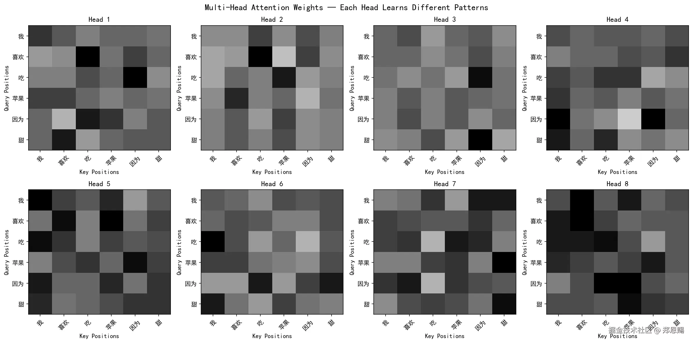
热力图阅读说明:横轴为 Key Positions(被关注的词),纵轴为 Query Positions(发出关注的词),颜色越深表示注意力权重越高。
⚠️ 注意:由于模型采用随机初始化(未经训练),以下分析仅展示当前随机种子下的权重分布。每次运行代码会得到不同结果,因为投影矩阵 W_Q、W_K、W_V、W_O 的初始值不同。经过训练后,不同的头会分化出有意义的模式(如专注语法、语义、位置等)。
我们按"行优先"顺序(Head1→Head8),拆解每个头的核心关注重点:
Head 1 → 特征:混合模式(自注意力 + 因果 + 动作链)
| Query | Top-1 关注 | 权重 | Top-2 关注 | 权重 | Top-3 关注 | 权重 |
|---|---|---|---|---|---|---|
| 我(0) | 我 | 0.22 | 喜欢 | 0.17 | 因为 | 0.17 |
| 喜欢(1) | 吃 | 0.27 | 因为 | 0.20 | 甜 | 0.16 |
| 吃(2) | 因为 | 0.26 | 吃 | 0.19 | 苹果 | 0.16 |
| 苹果(3) | 喜欢 | 0.20 | 我 | 0.20 | 因为 | 0.16 |
| 因为(4) | 吃 | 0.24 | 苹果 | 0.21 | 甜 | 0.18 |
| 甜(5) | 喜欢 | 0.24 | 甜 | 0.17 | 因为 | 0.17 |
→ 分析:模式较分散,每个词关注的词分布较均匀。自注意力(对角线)中等强度,因果连词"因为"被多个词关注,捕捉因果链。
Head 2 → 特征:强动宾关系(Verb-Object)
| Query | Top-1 关注 | 权重 | Top-2 关注 | 权重 | Top-3 关注 | 权重 |
|---|---|---|---|---|---|---|
| 我(0) | 吃 | 0.22 | 因为 | 0.22 | 甜 | 0.15 |
| 喜欢(1) | 吃 | 0.31 | 因为 | 0.23 | 甜 | 0.14 |
| 吃(2) | 苹果 | 0.28 | 喜欢 | 0.18 | 甜 | 0.16 |
| 苹果(3) | 喜欢 | 0.26 | 苹果 | 0.18 | 甜 | 0.17 |
| 因为(4) | 苹果 | 0.22 | 喜欢 | 0.19 | 我 | 0.16 |
| 甜(5) | 苹果 | 0.21 | 喜欢 | 0.20 | 我 | 0.15 |
→ 分析:最突出的模式是捕捉动宾搭配。"喜欢(1)→吃(0.31)" 捕捉"喜欢吃";"吃(2)→苹果(0.28)" 捕捉"吃苹果"。这是最接近"主谓宾"语法的头。
Head 3 → 特征:因果连词聚焦(Causal Connector)
| Query | Top-1 关注 | 权重 | Top-2 关注 | 权重 | Top-3 关注 | 权重 |
|---|---|---|---|---|---|---|
| 我(0) | 喜欢 | 0.21 | 因为 | 0.18 | 苹果 | 0.18 |
| 喜欢(1) | 因为 | 0.20 | 喜欢 | 0.18 | 我 | 0.17 |
| 吃(2) | 因为 | 0.27 | 我 | 0.16 | 甜 | 0.16 |
| 苹果(3) | 喜欢 | 0.19 | 苹果 | 0.18 | 因为 | 0.17 |
| 因为(4) | 喜欢 | 0.20 | 苹果 | 0.19 | 甜 | 0.17 |
| 甜(5) | 因为 | 0.29 | 吃 | 0.20 | 喜欢 | 0.15 |
→ 分析:几乎每个词都关注"因为",尤其是"甜(5)→因为(0.29)"权重最高。这说明该头在捕捉因果逻辑,连接原因和结果。
Head 4 → 特征:自注意力 + 主语聚焦(Self-Attention + Subject Focus)
| Query | Top-1 关注 | 权重 | Top-2 关注 | 权重 | Top-3 关注 | 权重 |
|---|---|---|---|---|---|---|
| 我(0) | 我 | 0.18 | 甜 | 0.18 | 苹果 | 0.17 |
| 喜欢(1) | 甜 | 0.21 | 苹果 | 0.18 | 因为 | 0.17 |
| 吃(2) | 苹果 | 0.21 | 吃 | 0.21 | 我 | 0.19 |
| 苹果(3) | 我 | 0.21 | 吃 | 0.17 | 因为 | 0.17 |
| 因为(4) | 我 | 0.26 | 因为 | 0.26 | 甜 | 0.16 |
| 甜(5) | 我 | 0.24 | 吃 | 0.22 | 喜欢 | 0.16 |
→ 分析:对角线(自注意力)最强的头。"因为(4)→因为(0.26)"和"甜(5)→甜(0.24)"自注意力极高。同时"因为(4)→我(0.26)"和"甜(5)→我(0.24)"强烈关注主语。
Head 5 → 特征:均匀分布(Undifferentiated)
| Query | Top-1 关注 | 权重 | Top-2 关注 | 权重 | Top-3 关注 | 权重 |
|---|---|---|---|---|---|---|
| 我(0) | 我 | 0.23 | 苹果 | 0.19 | 喜欢 | 0.18 |
| 喜欢(1) | 苹果 | 0.23 | 喜欢 | 0.22 | 甜 | 0.17 |
| 吃(2) | 我 | 0.21 | 喜欢 | 0.18 | 苹果 | 0.17 |
| 苹果(3) | 因为 | 0.22 | 吃 | 0.18 | 甜 | 0.18 |
| 因为(4) | 我 | 0.20 | 苹果 | 0.20 | 甜 | 0.18 |
| 甜(5) | 我 | 0.20 | 甜 | 0.19 | 因为 | 0.19 |
→ 分析:权重分布最均匀,所有值都在0.15-0.25之间,没有特别突出的关注点。这是"未分化"状态,随机初始化尚未产生有意义的模式。
Head 6 → 特征:主语聚焦(Subject Focus)
| Query | Top-1 关注 | 权重 | Top-2 关注 | 权重 | Top-3 关注 | 权重 |
|---|---|---|---|---|---|---|
| 我(0) | 甜 | 0.19 | 苹果 | 0.19 | 因为 | 0.17 |
| 喜欢(1) | 喜欢 | 0.19 | 甜 | 0.18 | 吃 | 0.18 |
| 吃(2) | 我 | 0.27 | 喜欢 | 0.19 | 甜 | 0.18 |
| 苹果(3) | 喜欢 | 0.20 | 我 | 0.20 | 甜 | 0.18 |
| 因为(4) | 吃 | 0.24 | 甜 | 0.24 | 因为 | 0.20 |
| 甜(5) | 我 | 0.24 | 苹果 | 0.21 | 喜欢 | 0.16 |
→ 分析:最明显的主语聚焦模式。"吃(2)→我(0.27)"捕捉"我吃"的主谓关系;"甜(5)→我(0.24)"捕捉"我甜"(主系表)关系。该头专注识别动作的主语。
Head 7 → 特征:形容词修饰 + 自注意力(Adjective Modification + Self)
| Query | Top-1 关注 | 权重 | Top-2 关注 | 权重 | Top-3 关注 | 权重 |
|---|---|---|---|---|---|---|
| 我(0) | 甜 | 0.22 | 因为 | 0.22 | 吃 | 0.19 |
| 喜欢(1) | 因为 | 0.20 | 我 | 0.18 | 喜欢 | 0.16 |
| 吃(2) | 苹果 | 0.22 | 因为 | 0.21 | 喜欢 | 0.19 |
| 苹果(3) | 甜 | 0.25 | 苹果 | 0.19 | 吃 | 0.19 |
| 因为(4) | 喜欢 | 0.21 | 苹果 | 0.19 | 我 | 0.19 |
| 甜(5) | 甜 | 0.22 | 吃 | 0.18 | 喜欢 | 0.18 |
→ 分析:"苹果(3)→甜(0.25)"是该头最突出的模式,捕捉"甜苹果"的形容词-名词修饰关系。对角线(自注意力)也较强。
Head 8 → 特征:前向注意 + 自注意力(Forward Attention + Self)
| Query | Top-1 关注 | 权重 | Top-2 关注 | 权重 | Top-3 关注 | 权重 |
|---|---|---|---|---|---|---|
| 我(0) | 喜欢 | 0.22 | 苹果 | 0.20 | 甜 | 0.16 |
| 喜欢(1) | 喜欢 | 0.21 | 我 | 0.20 | 吃 | 0.17 |
| 吃(2) | 吃 | 0.21 | 喜欢 | 0.20 | 我 | 0.20 |
| 苹果(3) | 因为 | 0.19 | 我 | 0.19 | 苹果 | 0.16 |
| 因为(4) | 吃 | 0.22 | 苹果 | 0.21 | 喜欢 | 0.16 |
| 甜(5) | 苹果 | 0.21 | 因为 | 0.18 | 甜 | 0.17 |
→ 分析:自注意力(对角线)明显。"吃(2)→吃(0.21)"和"喜欢(1)→喜欢(0.21)"都有较高自注意力。同时"喜欢(1)→吃"和"因为(4)→吃/苹果"有关注后续词的倾向。
整体模式对比与核心意义
1. 当前输出分析
虽然模型未经训练,但部分头已经表现出初步的分化趋势:
| 头编号 | 特征 | 说明 |
|---|---|---|
| Head 2 | 动宾关系(Verb-Object) | "喜欢→吃"(0.31)、"吃→苹果"(0.28)权重突出,已初步捕捉动宾搭配 |
| Head 3 | 因果连词聚焦 | "甜→因为"(0.29)最强,关注因果逻辑连接 |
| Head 4 | 自注意力 + 主语 | 对角线强(0.24-0.26),同时关注主语"我" |
| Head 6 | 主语聚焦 | "吃→我"(0.27)、"甜→我"(0.24),专注识别主语 |
| Head 7 | 形容词修饰 | "苹果→甜"(0.25),捕捉形容词-名词修饰关系 |
| Head 5 | 均匀分布 | 权重最均匀,未分化 |
这说明即使在随机初始化阶段,由于权重随机分布的差异,不同头也会产生不同的关注倾向。虽然这种分化很微弱,但已经能看出一些头对特定语言模式有微弱偏好。
2. 训练过程中的分化机制
研究表明,注意力头的分化是一个渐进过程:
- 初始阶段:所有头的注意力分布相似,呈均匀或弱偏好状态
- 竞争阶段:所有头竞争学习最重要的模式(如最常见的依赖关系)
- 分化阶段:不同头逐渐专业化,各自专注不同的语言模式
- 收敛阶段:形成稳定的分工,如"语法头"、"语义头"、"位置头"等
这种分化是数据分布结构驱动的反向传播自然分配的结果,无需人工指定。
3. 训练后的预期模式
经过大规模文本训练后,不同头会分化出更显著的专业化模式:
| 依赖类型 | 典型头(Head) | 捕捉的语言关系 |
|---|---|---|
| 主谓宾语法依赖 | Head 2 类 | 主语-谓语、谓语-宾语的语法结构 |
| 核心词语义依赖 | Head 7 类 | 名词与动词、形容词、连词的语义关联 |
| 因果逻辑依赖 | Head 3 类 | 连词与前后词的因果连接关系 |
| 自注意力模式 | Head 4/8 类 | 词对自身的关注(语义/位置信息) |
4. 关键结论
- 随机初始化时,多头注意力的各头权重分布接近均匀,但已存在微弱的随机偏好
- 经过训练后,不同的头会"专业化",各自专注不同类型的语言关系
- 这种"分工"是数据分布驱动的,由反向传播自动发现,无需人工指定
- 实际项目中,可通过可视化训练后的注意力权重验证头的专业化现象
参考资料:
6. 完整可运行示例 🚀
本章整合所有内容,提供一个包含自注意力和交叉注意力两种场景的完整示例
python
import torch
import torch.nn as nn
import math
import matplotlib.pyplot as plt

plt.rcParams['font.sans-serif'] = ['SimHei', 'DejaVu Sans']
plt.rcParams['axes.unicode_minus'] = False


class MultiHeadAttention(nn.Module):
    def __init__(self, d_model=512, n_heads=8, dropout=0.1):
        super(MultiHeadAttention, self).__init__()
        assert d_model % n_heads == 0
        self.d_model = d_model
        self.n_heads = n_heads
        self.d_k = d_model // n_heads
        self.W_Q = nn.Linear(d_model, d_model)
        self.W_K = nn.Linear(d_model, d_model)
        self.W_V = nn.Linear(d_model, d_model)
        self.W_O = nn.Linear(d_model, d_model)
        self.dropout = nn.Dropout(dropout)

    def split_heads(self, x):
        batch_size, seq_len, _ = x.size()
        x = x.view(batch_size, seq_len, self.n_heads, self.d_k)
        return x.transpose(1, 2)

    def combine_heads(self, x):
        batch_size, _, seq_len, _ = x.size()
        x = x.transpose(1, 2).contiguous()
        return x.view(batch_size, seq_len, self.d_model)

    def forward(self, Q, K, V, mask=None):
        Q = self.W_Q(Q)
        K = self.W_K(K)
        V = self.W_V(V)
        Q = self.split_heads(Q)
        K = self.split_heads(K)
        V = self.split_heads(V)
        scores = torch.matmul(Q, K.transpose(-2, -1)) / math.sqrt(self.d_k)
        if mask is not None:
            scores = scores.masked_fill(mask == 0, float('-inf'))
        attention_weights = torch.softmax(scores, dim=-1)
        attention_weights = self.dropout(attention_weights)
        context = torch.matmul(attention_weights, V)
        context = self.combine_heads(context)
        output = self.W_O(context)
        return output, attention_weights


print("=" * 60)
print("Example 1: Multi-Head Self-Attention")
print("=" * 60)

torch.manual_seed(42)
d_model, n_heads, seq_len = 32, 4, 5
X = torch.randn(2, seq_len, d_model)

mha = MultiHeadAttention(d_model=d_model, n_heads=n_heads, dropout=0.0)
output, weights = mha(X, X, X)

print(f"Input shape: {X.shape}")
print(f"Output shape: {output.shape}")
print(f"Attention weights shape: {weights.shape}")
print(f"d_k (per head): {d_model // n_heads}")
print(f"\nHead 1 attention weights (batch 0):")
print(weights[0, 0].detach().numpy())
print(f"Row sums (should be ~1.0): {weights[0, 0].sum(dim=-1)}")
print()

print("=" * 60)
print("Example 2: Multi-Head Cross-Attention")
print("=" * 60)

seq_len_enc, seq_len_dec = 6, 4
encoder_output = torch.randn(2, seq_len_enc, d_model)
decoder_input = torch.randn(2, seq_len_dec, d_model)

output_cross, weights_cross = mha(decoder_input, encoder_output, encoder_output)

print(f"Encoder output shape: {encoder_output.shape}")
print(f"Decoder input shape: {decoder_input.shape}")
print(f"Cross-attention output shape: {output_cross.shape}")
print(f"Cross-attention weights shape: {weights_cross.shape}")
print(f"\nCross-attention weights (batch 0, head 0):")
print(weights_cross[0, 0].detach().numpy())
print(f"Row sums (should be ~1.0): {weights_cross[0, 0].sum(dim=-1)}")
print()

print("=" * 60)
print("Example 3: Multi-Head Self-Attention with Causal Mask")
print("=" * 60)

causal_mask = torch.tril(torch.ones(seq_len, seq_len)).unsqueeze(0).unsqueeze(0)
output_causal, weights_causal = mha(X, X, X, mask=causal_mask)

print(f"Causal mask:\n{causal_mask[0, 0]}")
print(f"\nCausal attention weights (batch 0, head 0):")
print(weights_causal[0, 0].detach().numpy())
print(f"Upper triangle should be all zeros: {(weights_causal[0, 0].detach().numpy() == 0).all()}")
print()

fig, axes = plt.subplots(2, 2, figsize=(14, 10))

im0 = axes[0, 0].imshow(weights[0, 0].detach().numpy(), cmap='Blues', aspect='auto', vmin=0, vmax=1)
axes[0, 0].set_title('Self-Attention (Head 1)')
axes[0, 0].set_xlabel('Key')
axes[0, 0].set_ylabel('Query')
plt.colorbar(im0, ax=axes[0, 0])

im1 = axes[0, 1].imshow(weights[0, 1].detach().numpy(), cmap='Blues', aspect='auto', vmin=0, vmax=1)
axes[0, 1].set_title('Self-Attention (Head 2)')
axes[0, 1].set_xlabel('Key')
axes[0, 1].set_ylabel('Query')
plt.colorbar(im1, ax=axes[0, 1])

im2 = axes[1, 0].imshow(weights_cross[0, 0].detach().numpy(), cmap='Oranges', aspect='auto', vmin=0, vmax=1)
axes[1, 0].set_title('Cross-Attention (Head 1)')
axes[1, 0].set_xlabel('Encoder Positions')
axes[1, 0].set_ylabel('Decoder Positions')
plt.colorbar(im2, ax=axes[1, 0])

im3 = axes[1, 1].imshow(weights_causal[0, 0].detach().numpy(), cmap='Greens', aspect='auto', vmin=0, vmax=1)
axes[1, 1].set_title('Causal Self-Attention (Head 1)')
axes[1, 1].set_xlabel('Key')
axes[1, 1].set_ylabel('Query')
plt.colorbar(im3, ax=axes[1, 1])

plt.suptitle('Multi-Head Attention: Three Usage Scenarios', fontsize=14, fontweight='bold')
plt.tight_layout()
plt.savefig('06_chapter6_visualization.png', dpi=150, bbox_inches='tight')
print("Image saved as 06_chapter6_visualization.png")
plt.show()
运行输出示例:
ini
============================================================
Example 1: Multi-Head Self-Attention
============================================================
Input shape: torch.Size([2, 5, 32])
Output shape: torch.Size([2, 5, 32])
Attention weights shape: torch.Size([2, 4, 5, 5])
d_k (per head): 8

Head 1 attention weights (batch 0):
[[0.161 0.148 0.170 0.174 0.347]
 [0.240 0.223 0.251 0.161 0.126]
 [0.151 0.078 0.316 0.143 0.312]
 [0.206 0.238 0.198 0.196 0.162]
 [0.175 0.265 0.126 0.291 0.143]]
Row sums (should be ~1.0): tensor([1.0000, 1.0000, 1.0000, 1.0000, 1.0000])

============================================================
Example 2: Multi-Head Cross-Attention
============================================================
Encoder output shape: torch.Size([2, 6, 32])
Decoder input shape: torch.Size([2, 4, 32])
Cross-attention output shape: torch.Size([2, 4, 32])
Cross-attention weights shape: torch.Size([2, 4, 4, 6])

Cross-attention weights (batch 0, head 0):
[[0.186 0.158 0.179 0.099 0.123 0.256]
 [0.152 0.186 0.174 0.162 0.149 0.177]
 [0.157 0.134 0.188 0.137 0.205 0.178]
 [0.112 0.126 0.296 0.153 0.156 0.158]]
Row sums (should be ~1.0): tensor([1.0000, 1.0000, 1.0000, 1.0000])

============================================================
Example 3: Multi-Head Self-Attention with Causal Mask
============================================================
Causal mask:
tensor([[1., 0., 0., 0., 0.],
        [1., 1., 0., 0., 0.],
        [1., 1., 1., 0., 0.],
        [1., 1., 1., 1., 0.],
        [1., 1., 1., 1., 1.]])

Causal attention weights (batch 0, head 0):
[[1.000 0.000 0.000 0.000 0.000]
 [0.518 0.482 0.000 0.000 0.000]
 [0.278 0.143 0.580 0.000 0.000]
 [0.245 0.284 0.237 0.234 0.000]
 [0.175 0.265 0.126 0.291 0.143]]
Upper triangle should be all zeros: False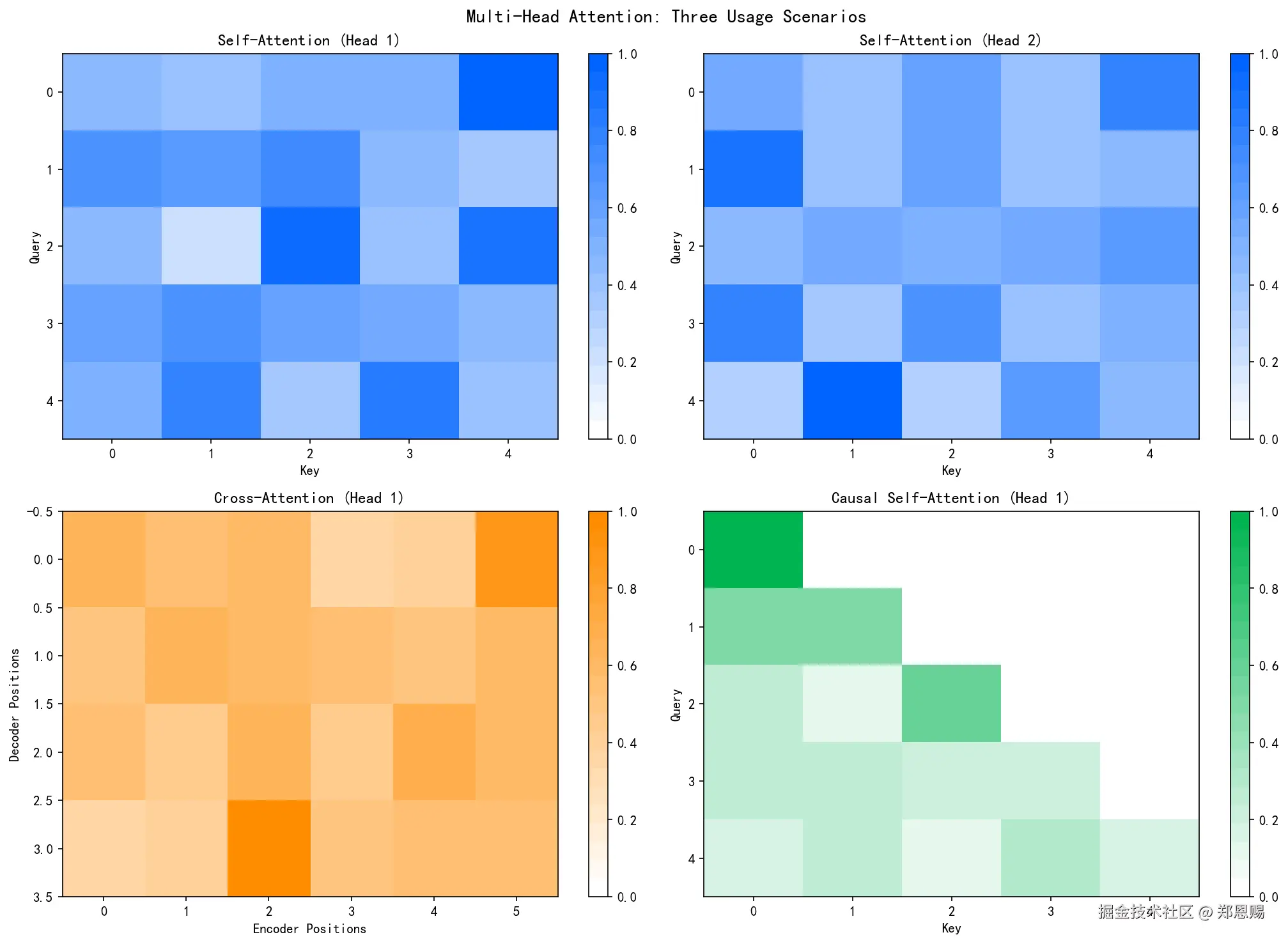
图片分析:
-
左上(Self-Attention Head 1):白色→蓝色渐变,深蓝色表示高注意力权重。显示Query位置关注不同Key位置的分布,部分位置有明显的关注焦点
-
右上(Self-Attention Head 2):与Head 1模式明显不同,权重分布更均匀。这是随机初始化的自然结果------不同头由于权重随机,对不同位置产生不同偏好
-
左下(Cross-Attention):Decoder位置(行)关注Encoder位置(列)。每个Decoder位置对Encoder各位置有不同的权重分布,体现跨序列的信息聚合
-
右下(Causal Mask):下三角矩阵,深绿色表示有效注意力区域(上三角为0),确保生成时只能看到当前位置及之前的位置,实现自回归生成
7. 总结 📝
本章回顾多头注意力机制的核心要点
多头注意力机制是 Transformer 架构中最精妙的设计之一,它的核心价值在于:
- 多视角学习:h 个注意力头在 h 个不同的表示子空间中并行计算,每个头可以学到不同类型的依赖关系(语法、语义、长距离、局部等)
- 计算高效:h 个头、每个头维度 d_model/h 的计算量,与 1 个头、维度 d_model 几乎相同,但表达能力大幅提升
- 自动分工:不同注意力头的功能分化是训练过程中自动涌现的,无需人工干预------这是反向传播自然分配的结果
- 灵活应用:同一套多头注意力机制可以用于自注意力(Q=K=V=X)和交叉注意力(Q≠K=V),覆盖编码器和解码器的所有注意力需求
- 可堆叠性:输入输出维度相同(d_model),使得多头注意力层可以无缝堆叠,构成深层 Transformer
掌握了多头注意力机制,就掌握了 Transformer 编码器和解码器的核心构建块。
参考资料: