文章目录
- Tensor
- CPU和GPU数据搬运
- dtype与内存:fp32、fp16、bf16
- 自动微分(autograd)
-
- 计算图
- [requires_grad 和 backward()](#requires_grad 和 backward())
- 梯度累计与清零
- 代码示例:手动梯度下降学习y=2x+1
- nn.Module:模型的组织方式
-
- [定义模型:继承nn.Module,实现_init_和 forward](#定义模型:继承nn.Module,实现_init_和 forward)
- [参数管理:parameters(), named_parameters(), state_dicct()](#参数管理:parameters(), named_parameters(), state_dicct())
- 完整训练循环
- GPU训练基础
- 性能分析
Tensor
如果把深度学习比作搭积木,Tensor 就是最基本的积木块。所有的模型参数、输入数据、中间计算结果,在 PyTorch 里都以 Tensor 的形式存在。
正式定义:Tensor(张量)是一个多维数组,可以看作 NumPy ndarray 的 GPU 加速版本,同时支持自动微分。
Tensor的常用方式
python
import torch
import numpy as np

a = torch.tensor([1.0, 2.0, 3.0])          # 从 Python 列表创建
zeros = torch.zeros(3, 4)                    # 3x4 全零矩阵
ones = torch.ones(2, 3, 4)                   # 2x3x4 全一张量
rand_normal = torch.randn(3, 4)              # 标准正态分布
seq = torch.arange(0, 10, 2)                 # tensor([0, 2, 4, 6, 8])

x = torch.randn(3, 4)
y = torch.zeros_like(x)                      # 和 x 形状一样的全零 Tensor

t = torch.from_numpy(np.array([1.0, 2.0]))   # 从 NumPy 转换(共享内存)
形状操作:view、reshape、permute、squeeze、unsqueeze
把 Tensor 想象成一块可以任意捏形的橡皮泥------数据不变,只是换个排列方式。
python
import torch

x = torch.arange(12)             # 一维,12 个元素
a = x.view(3, 4)                 # 变成 3x4(要求内存连续)
b = x.reshape(3, 4)              # 和 view 类似,但内存不连续时也能用
c = x.view(-1, 4)                # -1 自动推断为 3

# permute:交换维度,Transformer 中常用
t = torch.randn(2, 8, 12, 64)              # (batch, seq_len, heads, dim)
t_permuted = t.permute(0, 2, 1, 3)         # (batch, heads, seq_len, dim)

# squeeze/unsqueeze:去掉或插入大小为 1 的维度
e = torch.randn(1, 3, 1, 4)
print(e.squeeze().shape)                    # torch.Size([3, 4])
f = torch.randn(3, 4)
print(f.unsqueeze(0).shape)                 # torch.Size([1, 3, 4])
CPU和GPU数据搬运
python
import torch

print(torch.cuda.is_available())            # GPU 是否可用

x = torch.randn(3, 4)
x_gpu = x.to('cuda')                        # CPU → GPU(推荐写法)
x_gpu = x.cuda()                             # 等价简写
x_cpu = x_gpu.cpu()                          # GPU → CPU

# 直接在 GPU 上创建(避免多余的搬运)
x_gpu = torch.randn(3, 4, device='cuda')
CPU-GPU 数据搬运走 PCIe 总线,带宽远低于 GPU 显存带宽。频繁的 .cpu() 和 .cuda() 调用往往是隐蔽的性能瓶颈
dtype与内存:fp32、fp16、bf16
不同的数据精度直接决定显存占用和计算速度:
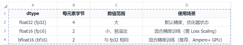
fp32 像高清照片,又大又清晰;fp16 像压缩照片,体积减半但偶尔"失真"(溢出);bf16 是聪明的压缩,体积和 fp16 一样小,但"失真"概率大大降低。
python
import torch

x_fp32 = torch.randn(1000, 1000, dtype=torch.float32)   # 4 bytes/element
x_bf16 = torch.randn(1000, 1000, dtype=torch.bfloat16)  # 2 bytes/element
print(f"fp32: {x_fp32.nelement() * x_fp32.element_size() / 1024:.0f} KB")  # 3906 KB
print(f"bf16: {x_bf16.nelement() * x_bf16.element_size() / 1024:.0f} KB")  # 1953 KB

x = torch.randn(3, 4)                     # 默认 fp32
x_half = x.half()                          # 转 fp16
x_bf16 = x.to(torch.bfloat16)             # 转 bf16
自动微分(autograd)
训练神经网络的核心是"根据损失调整参数",而调整的依据就是梯度。PyTorch 的 autograd 引擎帮你自动完成这件事。
计算图
计算图(Computational Graph)是一个有向无环图(DAG),节点代表 Tensor,边代表运算操作。PyTorch 在前向传播时动态构建图,反向传播时沿图计算梯度。PyTorch 采用动态计算图(Define-by-Run),支持 if/else、for 循环等 Python 控制流。
requires_grad 和 backward()
python
import torch

x = torch.tensor([2.0, 3.0], requires_grad=True)  # 追踪所有操作
y = x * 3
z = y.sum()        # z = 3*2 + 3*3 = 15
z.backward()       # 反向传播
print(x.grad)      # tensor([3., 3.]),dz/dx = 3
要点:backward() 只能对标量调用;叶节点才保存梯度;计算图用完即释放。
梯度累计与清零
PyTorch 默认累加梯度,不自动清零。就像一个计数器,每次 backward() 都往上加。标准训练循环里,每个 step 开始前必须清零------否则上一轮梯度会混进来。
python
import torch

x = torch.tensor([1.0], requires_grad=True)
(x * 2).sum().backward()
print(x.grad)         # tensor([2.])
(x * 3).sum().backward()
print(x.grad)         # tensor([5.]) ← 2+3,梯度被累加!
x.grad.zero_()        # 手动清零
(x * 4).sum().backward()
print(x.grad)         # tensor([4.]) ← 清零后正确
# 实际训练中用 optimizer.zero_grad() 一次性清零所有参数的梯度
代码示例:手动梯度下降学习y=2x+1
python
import torch

w = torch.tensor([0.0], requires_grad=True)
b = torch.tensor([0.0], requires_grad=True)
x_train = torch.tensor([1.0, 2.0, 3.0, 4.0])
y_train = torch.tensor([3.0, 5.0, 7.0, 9.0])

for epoch in range(100):
    loss = ((w * x_train + b - y_train) ** 2).mean()
    loss.backward()
    with torch.no_grad():
        w -= 0.01 * w.grad
        b -= 0.01 * b.grad
    w.grad.zero_()
    b.grad.zero_()

print(f"学到的模型: y = {w.item():.2f}x + {b.item():.2f}")
# 输出接近 y = 2.00x + 1.00
nn.Module:模型的组织方式
如果 Tensor 是积木块,nn.Module 就是积木的"说明书"------它定义了积木怎么拼接(前向传播),并帮你清点所有零件(参数管理)。
定义模型:继承nn.Module,实现_init_和 forward
python
import torch
import torch.nn as nn

class SimpleModel(nn.Module):
    def __init__(self, input_dim, hidden_dim, output_dim):
        super().__init__()
        self.linear1 = nn.Linear(input_dim, hidden_dim)
        self.relu = nn.ReLU()
        self.linear2 = nn.Linear(hidden_dim, output_dim)

    def forward(self, x):
        return self.linear2(self.relu(self.linear1(x)))

model = SimpleModel(784, 256, 10)
output = model(torch.randn(32, 784))    # 用 model(x),不要直接调用 forward
print(output.shape)                       # torch.Size([32, 10])
参数管理:parameters(), named_parameters(), state_dicct()
python
import torch.nn as nn

model = nn.Linear(10, 5)
for name, param in model.named_parameters():
    print(f"{name}: {param.shape}")   # weight: [5, 10], bias: [5]

# 统计参数量
total_params = sum(p.numel() for p in model.parameters())
print(f"参数量: {total_params}")       # 55

# state_dict 用于保存和加载模型
print(model.state_dict().keys())       # odict_keys(['weight', 'bias'])
完整训练循环
数据加载:Dataset和DataLoader
- Dataset:定义"数据集里有什么"和"怎么取一条数据"
- DataLoader:定义"怎么分 batch 喂给模型"(batching、shuffling、多进程加载)
python
import torch
from torch.utils.data import Dataset, DataLoader

class SimpleDataset(Dataset):
    def __init__(self, data, labels):
        self.data, self.labels = data, labels
    def __len__(self):
        return len(self.data)
    def __getitem__(self, idx):
        return self.data[idx], self.labels[idx]

dataset = SimpleDataset(torch.randn(1000, 784), torch.randint(0, 10, (1000,)))
loader = DataLoader(dataset, batch_size=64, shuffle=True,
                    num_workers=4, pin_memory=True, drop_last=True)
标准训练流程
每个 step 的核心五步:forward → loss → backward → optimizer.step → zero_grad
学习率调度
python
import torch

optimizer = torch.optim.AdamW(model.parameters(), lr=1e-3)
# 常用调度器
scheduler = torch.optim.lr_scheduler.StepLR(optimizer, step_size=10, gamma=0.1)
scheduler = torch.optim.lr_scheduler.CosineAnnealingLR(optimizer, T_max=100)
# 每个 epoch 结束后调用 scheduler.step()
Checkpoint保存与恢复
python
import torch

# 保存(模型 + 优化器 + 训练进度,断点恢复需要全部保存)
torch.save({
    'epoch': epoch, 'model_state_dict': model.state_dict(),
    'optimizer_state_dict': optimizer.state_dict(), 'loss': avg_loss,
}, 'checkpoint.pt')

# 加载
ckpt = torch.load('checkpoint.pt', weights_only=False)
model.load_state_dict(ckpt['model_state_dict'])
optimizer.load_state_dict(ckpt['optimizer_state_dict'])
代码示例:完整MNIST训练脚本
python
import torch
import torch.nn as nn
from torch.utils.data import DataLoader
from torchvision import datasets, transforms

# 超参数设置
batch_size, lr, num_epochs = 128, 1e-3, 5

# 自动选择设备:如果有 CUDA 就用 GPU,否则用 CPU
device = torch.device("cuda" if torch.cuda.is_available() else "cpu")


# 定义多层感知机模型
class MLP(nn.Module):
    def __init__(self):
        super().__init__()

        # 使用 Sequential 按顺序搭建网络
        self.net = nn.Sequential(
            nn.Flatten(),              # 将 28x28 的图像拉平成 784 维向量
            nn.Linear(784, 256),       # 全连接层:输入 784,输出 256
            nn.ReLU(),                 # ReLU 激活函数,引入非线性
            nn.Dropout(0.1),           # Dropout,随机丢弃 10% 神经元,防止过拟合
            nn.Linear(256, 10),        # 输出层:10 个类别,对应数字 0-9
        )

    def forward(self, x):
        # 前向传播
        return self.net(x)


def main():
    # 数据预处理:
    # ToTensor:将 PIL 图像转成 Tensor,并把像素值缩放到 [0, 1]
    # Normalize:使用 MNIST 数据集的均值和标准差进行标准化
    transform = transforms.Compose([
        transforms.ToTensor(),
        transforms.Normalize((0.1307,), (0.3081,))
    ])

    # 加载 MNIST 训练集
    train_set = datasets.MNIST(
        "./data",
        train=True,
        download=True,
        transform=transform
    )

    # 加载 MNIST 测试集
    test_set = datasets.MNIST(
        "./data",
        train=False,
        transform=transform
    )

    # 构建训练集 DataLoader
    train_loader = DataLoader(
        train_set,
        batch_size=batch_size,
        shuffle=True,                  # 训练集打乱顺序
        num_workers=2,                 # 使用 2 个子进程加载数据
        pin_memory=torch.cuda.is_available()
    )

    # 构建测试集 DataLoader
    test_loader = DataLoader(
        test_set,
        batch_size=batch_size,
        shuffle=False,                 # 测试集一般不需要打乱
        num_workers=2,
        pin_memory=torch.cuda.is_available()
    )

    # 创建模型并移动到 CPU/GPU
    model = MLP().to(device)

    # 定义损失函数:多分类交叉熵
    criterion = nn.CrossEntropyLoss()

    # 定义优化器:AdamW
    optimizer = torch.optim.AdamW(model.parameters(), lr=lr)

    # 学习率调度器:余弦退火
    scheduler = torch.optim.lr_scheduler.CosineAnnealingLR(
        optimizer,
        T_max=num_epochs
    )

    # 开始训练
    for epoch in range(num_epochs):
        model.train()                  # 设置为训练模式
        total_loss = 0

        # 遍历训练数据
        for images, labels in train_loader:
            # 将数据移动到 CPU/GPU
            images = images.to(device)
            labels = labels.to(device)

            # 清空上一轮梯度
            optimizer.zero_grad()

            # 前向传播,计算预测结果
            outputs = model(images)

            # 计算损失
            loss = criterion(outputs, labels)

            # 反向传播,计算梯度
            loss.backward()

            # 更新模型参数
            optimizer.step()

            # 累加 loss,用于后面打印平均损失
            total_loss += loss.item()

        # 每个 epoch 结束后更新学习率
        scheduler.step()

        # 验证模型
        model.eval()                   # 设置为评估模式
        correct = 0

        # 验证阶段不需要计算梯度
        with torch.no_grad():
            for images, labels in test_loader:
                images = images.to(device)
                labels = labels.to(device)

                # 获取模型输出
                outputs = model(images)

                # 取概率最大的类别作为预测结果
                preds = outputs.argmax(dim=1)

                # 统计预测正确的样本数量
                correct += (preds == labels).sum().item()

        # 计算测试集准确率
        acc = correct / len(test_set) * 100

        # 打印当前 epoch 的训练损失和测试准确率
        print(
            f"Epoch {epoch + 1}/{num_epochs} | "
            f"Loss: {total_loss / len(train_loader):.4f} | "
            f"Acc: {acc:.2f}%"
        )

        # 保存 checkpoint,方便后续恢复训练或加载模型
        torch.save({
            "epoch": epoch + 1,
            "model_state_dict": model.state_dict(),
            "optimizer_state_dict": optimizer.state_dict(),
        }, f"ckpt_ep{epoch + 1}.pt")


# Windows 下使用 DataLoader 多进程时必须加这一句
# 否则 num_workers > 0 时可能会报错或无限重启进程
if __name__ == "__main__":
    main()
GPU训练基础
将模型和数据搬到GPU
python
import torch
import torch.nn as nn

device = torch.device('cuda' if torch.cuda.is_available() else 'cpu')
model = nn.Linear(100, 10).to(device)
x = torch.randn(32, 100).to(device)     # 模型和数据必须在同一设备上
y = model(x)
混合精度训练入门
核心思路:前向和反向用低精度(fp16/bf16)加速计算,参数更新用高精度(fp32)保证精度。
python
import torch
import torch.nn as nn

device = torch.device('cuda')
model = nn.Sequential(nn.Linear(784, 256), nn.ReLU(), nn.Linear(256, 10)).to(device)
optimizer = torch.optim.AdamW(model.parameters(), lr=1e-3)

# BF16 混合精度(推荐,Ampere+ GPU,不需要 GradScaler)
for images, labels in train_loader:
    images, labels = images.to(device), labels.to(device)
    with torch.autocast(device_type='cuda', dtype=torch.bfloat16):
        loss = nn.functional.cross_entropy(model(images), labels)
    loss.backward()
    optimizer.step()
    optimizer.zero_grad()

# FP16 混合精度(需要 GradScaler 防止梯度下溢)
scaler = torch.cuda.amp.GradScaler()
for images, labels in train_loader:
    images, labels = images.to(device), labels.to(device)
    with torch.autocast(device_type='cuda', dtype=torch.float16):
        loss = nn.functional.cross_entropy(model(images), labels)
    scaler.scale(loss).backward()
    scaler.step(optimizer)
    scaler.update()
    optimizer.zero_grad()
显存查看
python
import torch

print(f"已分配: {torch.cuda.memory_allocated() / 1024**3:.2f} GB")
print(f"峰值:   {torch.cuda.max_memory_allocated() / 1024**3:.2f} GB")
print(torch.cuda.memory_summary(abbreviated=True))

# 分析某段代码的显存
torch.cuda.reset_peak_memory_stats()
# ... 运行目标代码 ...
print(f"峰值: {torch.cuda.max_memory_allocated() / 1024**3:.2f} GB")
性能分析
torch.profiler 能告诉你每个操作花了多少时间、GPU 利用率如何、哪里在空等数据。
常见性能问题模式:
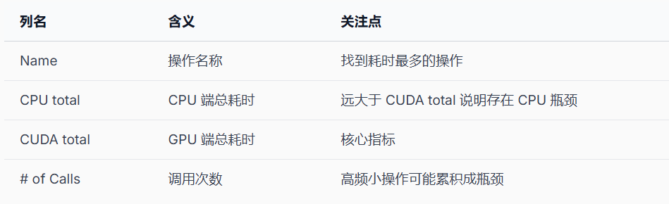
- CPU 时间远大于 CUDA 时间:GPU 在等 CPU(数据预处理、Python 开销)
- 大量小 CUDA kernel:launch overhead 累积,考虑 torch.compile 或算子融合
- 频繁 CPU-GPU 同步:.item()、print(tensor) 会触发同步,阻塞 GPU 流水线
常见性能问题
- 数据加载瓶颈:增加 num_workers,使用 prefetch_factor 预取数据。
- CPU-GPU 数据搬运:避免循环中反复 .cuda(),一次性搬运到 GPU。
- 隐式同步:loss.item() 触发 CPU-GPU 同步,应每 N 步才记录一次。
python
# 不好:每步都同步
for batch in dataloader:
    loss = train_step(batch)
    print(f"loss: {loss.item()}")       # 每步同步!

# 好:每 100 步记录一次
for i, batch in enumerate(dataloader):
    loss = train_step(batch)
    if i % 100 == 0:
        print(f"step {i}, loss: {loss.item()}")
代码示例:用profiler分析一个训练step
python
import torch
import torch.nn as nn
from torch.profiler import profile, record_function, ProfilerActivity
# 自动选择运行设备:
# 如果当前环境有可用 CUDA GPU,则使用 GPU;否则退回 CPU
device = torch.device("cuda" if torch.cuda.is_available() else "cpu")
# 定义一个较大的 MLP 模型
# 网络结构:
# 1024 -> 4096 -> ReLU -> 4096 -> ReLU -> 10
# 适合用来观察矩阵乘法、反向传播、优化器更新等耗时
model = nn.Sequential(
nn.Linear(1024, 4096),
nn.ReLU(),
nn.Linear(4096, 4096),
nn.ReLU(),
nn.Linear(4096, 10)
).to(device)
# 定义优化器
# AdamW 会维护一阶矩、二阶矩等状态,因此 optimizer_step 阶段会有一定开销
optimizer = torch.optim.AdamW(model.parameters(), lr=1e-3)
# 多分类交叉熵损失函数
criterion = nn.CrossEntropyLoss()
# 构造一批模拟输入数据
# data 形状为 [128, 1024],表示 batch size 为 128,每个样本 1024 维
data = torch.randn(128, 1024, device=device)
# 构造对应标签
# labels 形状为 [128],类别范围是 0 到 9
labels = torch.randint(0, 10, (128,), device=device)
# warmup:预热若干轮
# 第一次 CUDA 调用通常包含上下文初始化、kernel 加载等额外开销
# 预热后再 profiler,得到的性能数据更接近真实训练状态
for _ in range(3):
loss = criterion(model(data), labels)
loss.backward()
optimizer.step()
optimizer.zero_grad()
# 启动 PyTorch Profiler
# activities 同时记录 CPU 和 CUDA 活动
# record_shapes=True 记录算子的输入形状,方便分析张量维度
# profile_memory=True 记录 CPU/GPU 内存分配情况
with profile(
activities=[ProfilerActivity.CPU, ProfilerActivity.CUDA],
record_shapes=True,
profile_memory=True
) as prof:
# 自定义性能区间:数据创建与拷贝到 GPU
# 如果 device 是 cuda,这里会包含 CPU 创建随机数据 + 拷贝到 GPU 的开销
# 如果 device 是 cpu,则 .to(device) 基本不会产生 GPU 拷贝
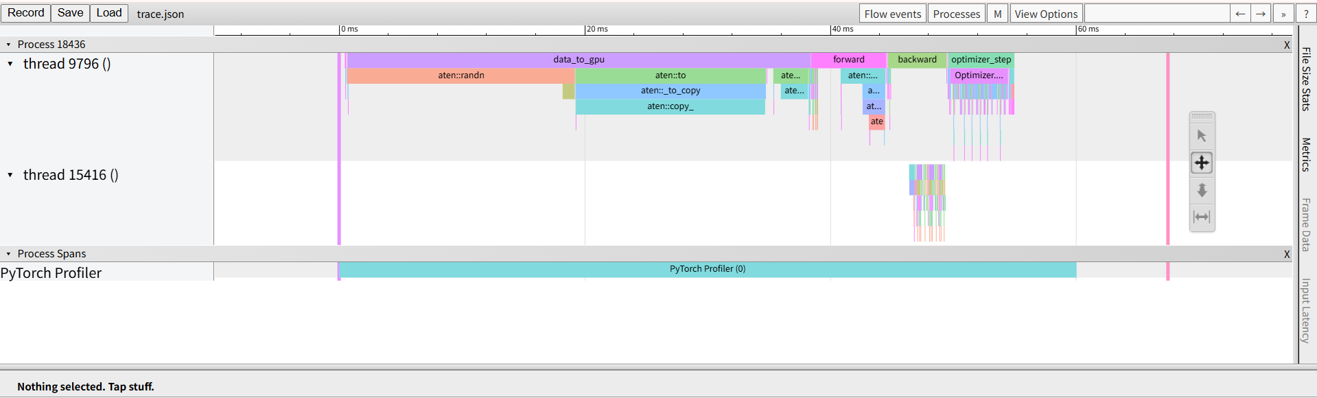
with record_function("data_to_gpu"):
d = torch.randn(128, 1024).to(device)
l = torch.randint(0, 10, (128,)).to(device)
# 自定义性能区间:前向传播
# 包括 Linear、ReLU、CrossEntropyLoss 等操作
with record_function("forward"):
loss = criterion(model(d), l)
# 自定义性能区间:反向传播
# 计算各层参数的梯度
with record_function("backward"):
loss.backward()
# 自定义性能区间:优化器更新
# AdamW 根据梯度更新参数,并清空梯度
with record_function("optimizer_step"):
optimizer.step()
optimizer.zero_grad()
# 打印 profiler 汇总表
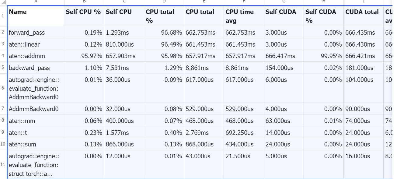
# 按 CUDA 总耗时排序,最多显示前 15 行
print(
prof.key_averages().table(
sort_by="cuda_time_total",
row_limit=15
)
)
# 导出 Chrome tracing 格式文件
# 可以在 chrome://tracing 或 Perfetto 中打开查看时间线
prof.export_chrome_trace("trace.json")