告别手动计算，SymPy 初识与 Manim 联动

下面是我正在做的一个抛物线演示动画。

需求很简单：展示一个二次函数 <math xmlns="http://www.w3.org/1998/Math/MathML"> y = x 2 − 2 x − 1 y = x^2 - 2x - 1 </math>y=x2−2x−1 的图像，并在上面标注几个关键点。

问题来了：

当我想调整函数参数时（比如把 <math xmlns="http://www.w3.org/1998/Math/MathML"> − 2 x -2x </math>−2x 改成 <math xmlns="http://www.w3.org/1998/Math/MathML"> − 3 x -3x </math>−3x），所有点的坐标都要手动重算
计算 <math xmlns="http://www.w3.org/1998/Math/MathML"> x = 1.5 x=1.5 </math>x=1.5 时的函数值？掏出计算器 → <math xmlns="http://www.w3.org/1998/Math/MathML"> 1. 5 2 − 2 × 1.5 − 1 = − 1.75 1.5^2 - 2×1.5 - 1 = -1.75 </math>1.52−2×1.5−1=−1.75 → 再手动填回代码
顶点坐标？求导 → 令导数等于0 → 解方程 → 计算 y 值 → 再填回代码
对称轴和 x 轴的交点？求根公式 → 计算器 → 填代码

一个参数改动，我要重新计算七八个坐标值。这哪是在做动画，分明是在做数学作业！

直到我发现了 SymPy 这个神器。

SymPy 是什么？为什么 Manim 动画需要它？

简单说，SymPy 是一个 Python 的符号计算库。

别被"符号计算"这个词吓到，用大白话讲就是：

让计算机帮你"列式子、解方程、求导数"，而不是你自己手算。

数值计算 vs 符号计算

看一个更直观的对比，你会立刻明白符号计算的强大：

python 复制代码

import math
import sympy as sp

# ========== 场景：计算 sin(π/3) 的精确值 ==========
# 数值计算 - 得到近似小数
result_num = math.sin(math.pi / 3)
print(f"数值计算: {result_num}")  
# 输出: 0.8660254037844386  ← 这是近似值，不知道它等于 √3/2

# 符号计算 - 得到精确表达式
x = sp.Symbol('x')
result_sym = sp.sin(sp.pi / 3)
print(f"符号计算: {result_sym}")  
# 输出: sqrt(3)/2  ← 精确的数学表达式！


# 场景1：求平方
print("\n=== 求 (sin(π/3))² ===")
# 数值计算 - 精度损失
square_num = result_num ** 2
print(f"数值: {square_num}")  
# 输出: 0.7499999999999999  ← 本应是 0.75，有浮点误差！

# 符号计算 - 精确化简
square_sym = result_sym ** 2
print(f"符号: {square_sym}")  
# 输出: 3/4  ← 精确值！

关键对比总结

特性	数值计算 (math)	符号计算 (sympy)
`sin(π/3)`	`0.86602540378...`	`√3/2`
平方后	`0.749999999999...`	`3/4`
能否继续代数运算	❌ 只能数值近似	✅ 可代入方程、求导、化简
浮点精度问题	⚠️ 存在误差累积	✅ 完全精确

符号计算的灵活性体现在：

保持数学形式 ：√3/2 比 0.866... 更有数学意义
自动化简 ：(√3/2)² 自动变成 3/4
代数兼容：可以继续解方程、求导、积分，保持精确形式

这对 Manim 动画尤为重要------你不仅需要坐标值，更需要数学关系的可视化，而符号计算保留了这种关系！

避免累积误差

符号计算在累积的计算中，能够有效的降低误差。

比如公式： <math xmlns="http://www.w3.org/1998/Math/MathML"> I n = 1 − n × I n − 1 I_n =1-n\times I_{n-1} </math>In=1−n×In−1其中 <math xmlns="http://www.w3.org/1998/Math/MathML"> I 0 = e − 1 I_0 = e-1 </math>I0=e−1。分别累积计算以后：

<math xmlns="http://www.w3.org/1998/Math/MathML"> n n </math>n	符号计算	数值计算 (模拟8位小数精度)	误差分析
0	<math xmlns="http://www.w3.org/1998/Math/MathML"> e − 1 e - 1 </math>e−1	0.71828183	初始误差： <math xmlns="http://www.w3.org/1998/Math/MathML"> ≈ 1.5 × 1 0 − 9 \approx 1.5 \times 10^{-9} </math>≈1.5×10−9
1	<math xmlns="http://www.w3.org/1998/Math/MathML"> 2 − e 2 - e </math>2−e	0.28171817	误差微小
2	<math xmlns="http://www.w3.org/1998/Math/MathML"> 2 e − 5 2e - 5 </math>2e−5	0.43656366	误差开始累积
3	<math xmlns="http://www.w3.org/1998/Math/MathML"> 16 − 6 e 16 - 6e </math>16−6e	0.30860902
4	<math xmlns="http://www.w3.org/1998/Math/MathML"> 24 e − 65 24e - 65 </math>24e−65	0.23687292
5	<math xmlns="http://www.w3.org/1998/Math/MathML"> 326 − 120 e 326 - 120e </math>326−120e	0.18276460	误差开始显现
6	<math xmlns="http://www.w3.org/1998/Math/MathML"> 1956 e − 5315 1956e - 5315 </math>1956e−5315	0.15054840
7	<math xmlns="http://www.w3.org/1998/Math/MathML"> 13692 − 5040 e 13692 - 5040e </math>13692−5040e	0.12145720
8	<math xmlns="http://www.w3.org/1998/Math/MathML"> 109536 e − 298325 109536e - 298325 </math>109536e−298325	0.10364240
9	<math xmlns="http://www.w3.org/1998/Math/MathML"> 985824 − 2691360 e 985824 - 2691360e </math>985824−2691360e	0.08385840
10	<math xmlns="http://www.w3.org/1998/Math/MathML"> 26913600 e − 73309365 26913600e - 73309365 </math>26913600e−73309365	0.07515840	偏差明显
11	<math xmlns="http://www.w3.org/1998/Math/MathML"> 296049600 − 807408000 e 296049600 - 807408000e </math>296049600−807408000e	0.09173440
12	<math xmlns="http://www.w3.org/1998/Math/MathML"> 9688896000 e − 26384952005 9688896000e - 26384952005 </math>9688896000e−26384952005	-0.08345440	灾难性错误：符号反转！
13	<math xmlns="http://www.w3.org/1998/Math/MathML"> 342938611200 − 1258293216000 e 342938611200 - 1258293216000e </math>342938611200−1258293216000e	2.10490720	完全失控

使用Sympy的话，可以在需要某一步结果的时候再代入 <math xmlns="http://www.w3.org/1998/Math/MathML"> e e </math>e去具体计算出来，不会累积误差。

SymPy 核心入门：把变量当作"符号"

在 SymPy 中，我们首先要定义符号变量：

python 复制代码

import sympy as sp

# 定义符号 - 告诉 SymPy "x 是一个数学变量，不是具体的数"
x = sp.Symbol('x')
y = sp.Symbol('y')

# 现在可以构建表达式了
expr = x**2 - 2*x - 1  # y = x² - 2x - 1
print(expr)  # 输出: x**2 - 2*x - 1

核心操作：代入求值 `.subs()`

有了表达式，我们可以轻松计算任意 x 对应的 y 值：

python 复制代码

# 计算 x=1.5 时的函数值
result = expr.subs(x, 1.5)
print(result)  # 输出: -1.75000000000000
print(float(result))  # 转换为浮点数: -1.75

自动求导和解方程

这才是真正解放双手的功能：

python 复制代码

# 求导数
derivative = sp.diff(expr, x)  # 对 x 求导
print(derivative)  # 输出: 2*x - 2

# 解方程：导数=0（找顶点）
vertex_x = sp.solve(derivative, x)[0]  # 解得 x=1
vertex_y = expr.subs(x, vertex_x)      # 代入求 y
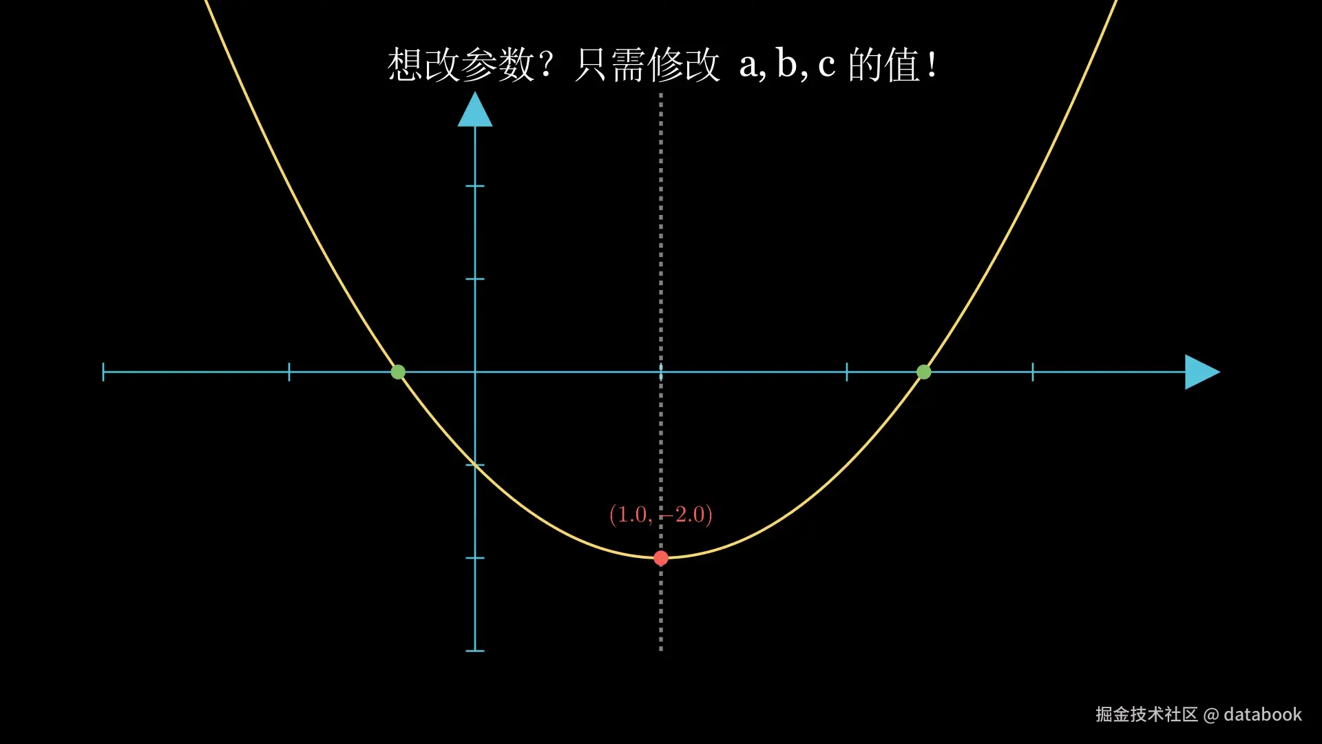
print(f"顶点坐标: ({vertex_x}, {vertex_y})")  # 输出: (1, -2)

# 解方程：y=0（找与x轴交点）
roots = sp.solve(expr, x)
print(f"与x轴交点: {roots}")  # 输出: [1 - sqrt(2), 1 + sqrt(2)]

看到了吗？ 原本需要手动计算的所有值，现在 SymPy 全自动搞定了！

SymPy 和 Manim 结合示例

现在我们把 SymPy 和 Manim 结合起来，做一个参数可调的抛物线动画。

核心代码示例

python 复制代码

from manim import *
import sympy as sp

class AutoParabola(Scene):
    def construct(self):
        # ========== SymPy 自动计算部分 ==========
        x = sp.Symbol('x')
        a, b, c = 1, -2, -1                      # 抛物线参数：y = ax² + bx + c
        expr = a * x**2 + b * x + c              # SymPy 符号表达式

        # 自动求顶点：令导数为 0
        derivative = sp.diff(expr, x)            # 求导：2ax + b
        vertex_x = float(sp.solve(derivative, x)[0])
        vertex_y = float(expr.subs(x, vertex_x))

        # 自动求与 x 轴交点
        roots = sp.solve(expr, x)                # 解方程 ax² + bx + c = 0
        root_points = [(float(r), 0) for r in roots if r.is_real]
        
        # ========== Manim 可视化部分 ==========
        axes = Axes(x_range=[-2, 4, 1], y_range=[-3, 3, 1], axis_config={"color": BLUE})
        
        # 用 SymPy 表达式直接作为绘图函数
        parabola = axes.plot(
            lambda x_val: float(expr.subs(x, x_val)),  # SymPy 实时计算 y 值
            color=YELLOW, stroke_width=3,
        )
        
        # 顶点（使用 SymPy 算出的坐标）
        vertex_dot = Dot(axes.c2p(vertex_x, vertex_y), color=RED)
        vertex_label = MathTex(
            f"({vertex_x:.1f}, {vertex_y:.1f})", font_size=24, color=RED
        ).next_to(vertex_dot, UP)

        # x 轴交点
        root_dots = VGroup(*[
            Dot(axes.c2p(rx, ry), color=GREEN) for rx, ry in root_points
        ])

        # ========== 动画播放 ==========
        self.play(Create(axes))
        self.play(Create(parabola))
        self.play(Create(vertex_dot), Write(vertex_label))
        self.play(Create(root_dots))
        self.wait(2)

代码核心解析

关键点1：无缝衔接

python 复制代码

# SymPy 计算出的值是符号类型，需要转为 float 给 Manim 使用
vertex_x = float(sp.solve(derivative, x)[0])

关键点2：动态函数映射

python 复制代码

# 用 lambda 将 SymPy 表达式"翻译"成 Manim 能理解的数值函数
parabola = axes.plot(
    lambda x_val: float(expr.subs(x, x_val)),
    color=YELLOW,
)

关键点3：坐标系转换

python 复制代码

# 数学坐标 → 屏幕坐标
vertex_dot = Dot(axes.c2p(vertex_x, vertex_y))

效果展示说明

运行这段代码后，你会看到：

坐标轴自动建立，范围根据函数特点自适应
抛物线精确绘制，形状由 SymPy 实时计算
红色顶点自动标注在正确位置，坐标值精确显示
绿色交点标记出抛物线与 x 轴的交点
白色虚线标出对称轴位置

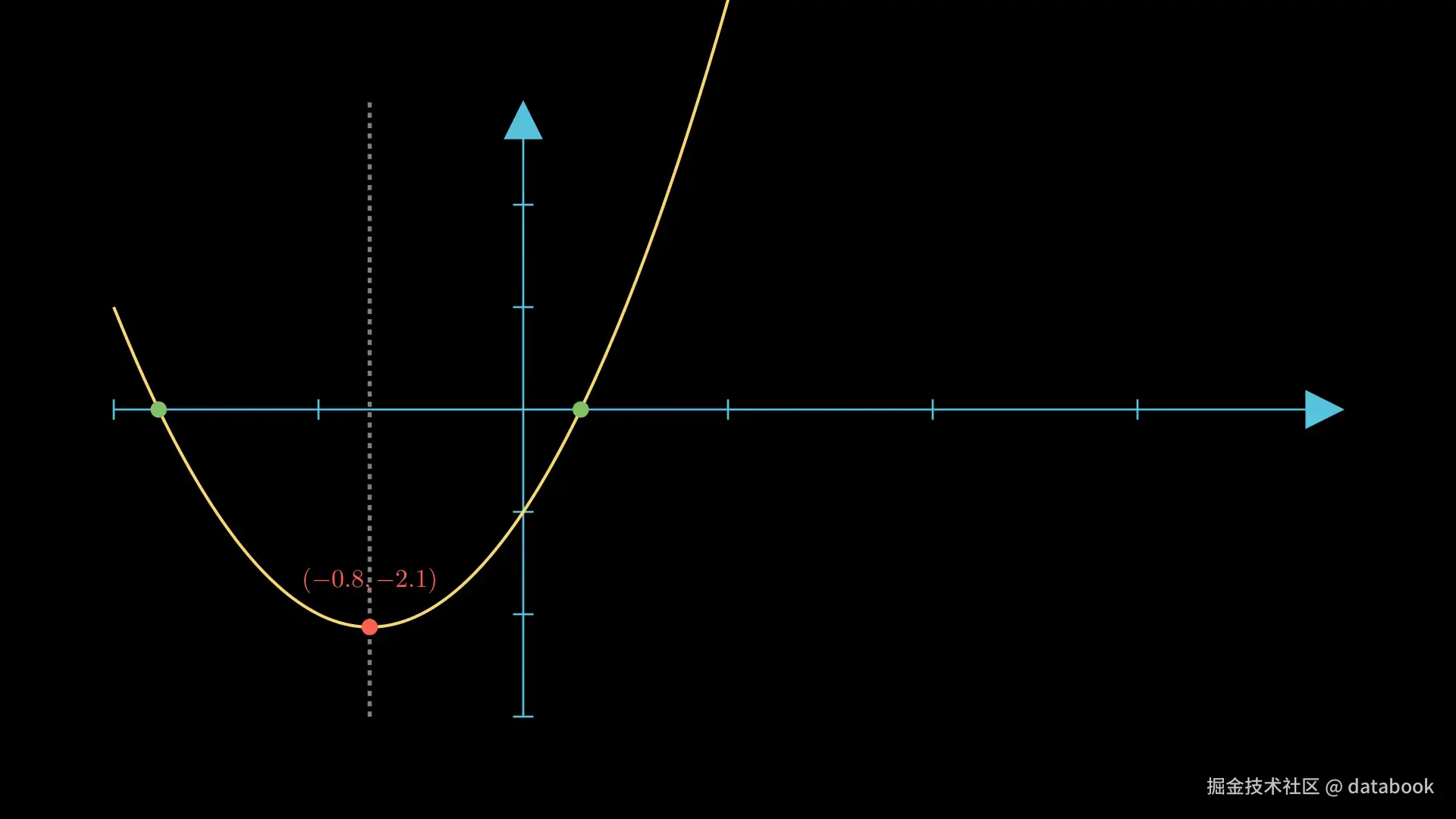
最神奇的是 ：如果你想改成 <math xmlns="http://www.w3.org/1998/Math/MathML"> y = 2 x 2 + 3 x − 1 y = 2x^2 + 3x - 1 </math>y=2x2+3x−1，只需要修改第 11 行的参数：

python 复制代码

a, b, c = 2, 3, -1  # 其他代码完全不用动！

所有的点、线、标注都会自动更新到正确位置！修改后：

小结

今天我们解决了 Manim 动画制作中的一大痛点：手动计算坐标。

通过 SymPy 的符号计算能力，我们实现了：

✅ 表达式精确计算：告别计算器
✅ 适合数学思维表达：将公式推导直接映射成代码
✅ 自动求导找顶点：告别手算求导
✅ 自动解方程找交点：告别求根公式
✅ 等等... ...

核心代码模板：

python 复制代码

import sympy as sp
x = sp.Symbol('x')
expr = x**2 - 2*x - 1  # 你的表达式
y_value = float(expr.subs(x, x_value))  # 计算任意点的值

告别手动计算，SymPy 初识与 Manim 联动

SymPy 是什么？为什么 Manim 动画需要它？

数值计算 vs 符号计算

避免累积误差

SymPy 核心入门：把变量当作"符号"

核心操作：代入求值 .subs()

自动求导和解方程

SymPy 和 Manim 结合示例

核心代码示例

代码核心解析

效果展示说明

小结

核心操作：代入求值 `.subs()`