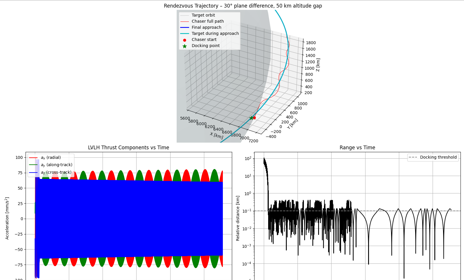
摘要:本文实现了一个基于LQR控制的航天器交会对接仿真系统。系统模拟了初始高度差50km、轨道平面倾角差30°的追踪航天器向目标航天器的自主接近过程。通过求解连续时间代数Riccati方程设计最优控制器,采用四阶龙格库塔法进行轨道动力学积分,并实现了LVLH坐标系下的相对运动控制。仿真结果显示系统能在5个轨道周期内完成对接,最终相对距离小于100米,速度差小于1m/s。可视化部分展示了3D轨迹、推力分量时域曲线和相对距离对数变化图,验证了控制算法的有效性。
python
import numpy as np
from scipy.linalg import solve_continuous_are
import matplotlib.pyplot as plt
from mpl_toolkits.mplot3d import Axes3D

# =============================================================================
# Constants and orbit parameters
# =============================================================================
mu = 3.986004418e5       # Earth gravitational parameter [km^3/s^2]
R_earth = 6371.0         # Earth radius [km]

# Target: circular equatorial orbit at 400 km altitude
a_t = R_earth + 400.0            # semi-major axis [km]
i_t = 0.0                        # equatorial plane
n   = np.sqrt(mu / a_t**3)       # mean motion [rad/s]
T   = 2*np.pi / n

# Chaser: 50 km higher orbit, plane inclined by 30 deg relative to equator
a_c = a_t + 50.0                 # 50 km altitude difference
i_c = np.deg2rad(30.0)           # 30 deg plane inclination difference

# Initial true anomalies (both at ascending node at t=0)
f0_t = 0.0
f0_c = 0.0

# =============================================================================
# Orbit propagation utilities
# =============================================================================
def oe2eci(a, e, inc, raan, argp, f):
    """Convert Keplerian orbital elements to ECI position and velocity."""
    r_pf = a * (1 - e**2) / (1 + e*np.cos(f))
    p_pf = np.array([r_pf*np.cos(f), r_pf*np.sin(f), 0.0])
    v_pf = np.sqrt(mu/(a*(1 - e**2))) * np.array([-np.sin(f), e+np.cos(f), 0.0])

    R_raan = np.array([[np.cos(raan), -np.sin(raan), 0],
                       [np.sin(raan),  np.cos(raan), 0],
                       [0,             0,            1]])
    R_inc  = np.array([[1, 0,             0],
                       [0, np.cos(inc), -np.sin(inc)],
                       [0, np.sin(inc),  np.cos(inc)]])
    R_argp = np.array([[np.cos(argp), -np.sin(argp), 0],
                       [np.sin(argp),  np.cos(argp), 0],
                       [0,             0,            1]])
    R = R_raan @ R_inc @ R_argp
    return R @ p_pf, R @ v_pf

def lvlh_basis(r, v):
    """Return rotation matrix from ECI to LVLH (rows are basis vectors)."""
    e_x = r / np.linalg.norm(r)
    h   = np.cross(r, v)
    e_z = h / np.linalg.norm(h)
    e_y = np.cross(e_z, e_x)
    return np.vstack([e_x, e_y, e_z])

# Initial states
r_t0, v_t0 = oe2eci(a_t, 0.0, i_t, 0.0, 0.0, f0_t)
r_c0, v_c0 = oe2eci(a_c, 0.0, i_c, 0.0, 0.0, f0_c)

# =============================================================================
# LQR controller design based on target circular orbit
# =============================================================================
A = np.zeros((6,6))
A[0,3] = 1.0
A[1,4] = 1.0
A[2,5] = 1.0
A[3,0] = 3*n**2
A[3,4] = 2*n
A[4,3] = -2*n
A[5,2] = -n**2
B = np.zeros((6,3))
B[3,0] = B[4,1] = B[5,2] = 1.0

# Tuning: larger penalty on state, smaller on control to handle large initial offset
Q = np.diag([1.0, 1.0, 1.0, 0.5, 0.5, 0.5])
R = np.diag([1e2, 1e2, 1e2])        # allow larger control acceleration
S = solve_continuous_are(A, B, Q, R)
K = np.linalg.inv(R) @ B.T @ S

# =============================================================================
# Simulation settings
# =============================================================================
dt = 5.0                   # integration step [s]
tmax = 5.0 * T             # allow up to 5 orbits for convergence
dock_dist = 0.1            # km
dock_vel  = 0.001          # km/s
thrust_limit = 0.1         # km/s^2 (approx 10 g) -- prevent numerical blow-up

r_c, v_c = r_c0.copy(), v_c0.copy()
t = 0.0

t_hist, r_c_hist, r_t_hist, u_lvlh_hist = [], [], [], []

while t < tmax:
    # Target state
    f_t = f0_t + n*t
    r_t, v_t = oe2eci(a_t, 0.0, i_t, 0.0, 0.0, f_t)

    # Relative state in LVLH
    R_lvlh = lvlh_basis(r_t, v_t)
    dr_eci = r_c - r_t
    dv_eci = v_c - v_t
    rho     = R_lvlh @ dr_eci
    rho_dot = R_lvlh @ dv_eci - np.cross([0,0,n], rho)
    x_lvlh = np.concatenate([rho, rho_dot])

    # Control in LVLH (clipped)
    u_lvlh_raw = -K @ x_lvlh
    u_norm = np.linalg.norm(u_lvlh_raw)
    if u_norm > thrust_limit:
        u_lvlh = u_lvlh_raw * (thrust_limit / u_norm)
    else:
        u_lvlh = u_lvlh_raw
    u_eci = R_lvlh.T @ u_lvlh

    # Log data
    t_hist.append(t)
    r_c_hist.append(r_c.copy())
    r_t_hist.append(r_t.copy())
    u_lvlh_hist.append(u_lvlh.copy())

    # Check docking condition
    if np.linalg.norm(dr_eci) < dock_dist and np.linalg.norm(dv_eci) < dock_vel:
        print(f"Docking achieved at t = {t:.1f} s")
        break

    # RK4 integration of chaser (full two-body + control)
    def accel(r, v, u):
        return -mu * r / np.linalg.norm(r)**3 + u
    k1v = v_c
    k1a = accel(r_c, v_c, u_eci)
    k2v = v_c + 0.5*dt*k1a
    k2a = accel(r_c + 0.5*dt*k1v, k2v, u_eci)
    k3v = v_c + 0.5*dt*k2a
    k3a = accel(r_c + 0.5*dt*k2v, k3v, u_eci)
    k4v = v_c + dt*k3a
    k4a = accel(r_c + dt*k3v, k4v, u_eci)
    r_c += dt/6 * (k1v + 2*k2v + 2*k3v + k4v)
    v_c += dt/6 * (k1a + 2*k2a + 2*k3a + k4a)
    t += dt

# Convert to arrays
t_arr = np.array(t_hist)
r_c_arr = np.array(r_c_hist)
r_t_arr = np.array(r_t_hist)
u_lvlh_arr = np.array(u_lvlh_hist)

# =============================================================================
# Visualization
# =============================================================================
plt.rcParams.update({'font.size': 10})
fig = plt.figure(figsize=(16, 12))

# ---- 3D trajectory with zoom on final approach ----
ax1 = fig.add_subplot(2, 2, (1,2), projection='3d')
# Earth globe
u = np.linspace(0, 2*np.pi, 40)
v = np.linspace(0, np.pi, 20)
x_e = R_earth * np.outer(np.cos(u), np.sin(v))
y_e = R_earth * np.outer(np.sin(u), np.sin(v))
z_e = R_earth * np.outer(np.ones_like(u), np.cos(v))
ax1.plot_surface(x_e, y_e, z_e, color='lightblue', alpha=0.15, edgecolor='none')

# Target orbit (full circle)
f_plot = np.linspace(0, 2*np.pi, 300)
r_target_orbit = np.array([oe2eci(a_t,0,i_t,0,0,f)[0] for f in f_plot])
ax1.plot(r_target_orbit[:,0], r_target_orbit[:,1], r_target_orbit[:,2],
         'gray', linestyle=':', linewidth=0.8, label='Target orbit')

# Chaser trajectory (full)
ax1.plot(r_c_arr[:,0], r_c_arr[:,1], r_c_arr[:,2],
         'r-', linewidth=0.8, label='Chaser full path')

# Highlight final approach segment (last 20% of data points)
n_approach = max(len(r_c_arr)//5, 2)
ax1.plot(r_c_arr[-n_approach:,0], r_c_arr[-n_approach:,1], r_c_arr[-n_approach:,2],
         'b-', linewidth=2.0, label='Final approach')
ax1.plot(r_t_arr[-n_approach:,0], r_t_arr[-n_approach:,1], r_t_arr[-n_approach:,2],
         'c-', linewidth=2.0, label='Target during approach')

# Markers
ax1.scatter(*r_c_arr[0],  c='red', marker='o', s=40, label='Chaser start')
ax1.scatter(*r_c_arr[-1], c='green', marker='*', s=100, label='Docking point')

# Zoom box around the target at final time
center = r_t_arr[-1]
span = 80.0   # km
ax1.set_xlim(center[0]-span, center[0]+span)
ax1.set_ylim(center[1]-span, center[1]+span)
ax1.set_zlim(center[2]-span, center[2]+span)
ax1.set_xlabel('X [km]'); ax1.set_ylabel('Y [km]'); ax1.set_zlabel('Z [km]')
ax1.set_title('Rendezvous Trajectory -- 30° plane difference, 50 km altitude gap')
ax1.legend(loc='upper left')

# ---- Thrust vs time (LVLH components) ----
ax2 = fig.add_subplot(2, 2, 3)
ax2.plot(t_arr, u_lvlh_arr[:,0]*1e3, 'r-', label='$a_x$ (radial)')
ax2.plot(t_arr, u_lvlh_arr[:,1]*1e3, 'g-', label='$a_y$ (along-track)')
ax2.plot(t_arr, u_lvlh_arr[:,2]*1e3, 'b-', label='$a_z$ (cross-track)')
ax2.set_xlabel('Time [s]')
ax2.set_ylabel('Acceleration [mm/s$^2$]')
ax2.set_title('LVLH Thrust Components vs Time')
ax2.legend(); ax2.grid(True)

# ---- Relative range (log scale) ----
ax3 = fig.add_subplot(2, 2, 4)
dist = np.linalg.norm(r_c_arr - r_t_arr, axis=1)
ax3.semilogy(t_arr, dist, 'k-')
ax3.axhline(y=dock_dist, color='gray', linestyle='--', label='Docking threshold')
ax3.set_xlabel('Time [s]')
ax3.set_ylabel('Relative distance [km]')
ax3.set_title('Range vs Time')
ax3.legend(); ax3.grid(True)

plt.tight_layout()
plt.show()