神经网络 替代 线性模型_进行模型学习

神经网络 替代 线性模型

深度学习的核心是神经网络： 一种能够通过简单函数的组合来表示复杂函数的数学实体。但现代人工神经网络与大脑中神经元的机制只有细微的相似之处。人工神经网络和生理神经网络似乎都使用模糊相似的数学策略来逼近复杂的函数，因为这类策略非常有效。

这些复杂函数的基本构建是神经元。其核心就是输入的线性变换（例如，将输入乘以一个数字【权重】，加上一个常数【偏置】），然后应用一个固定的非线性函数，即激活函数。

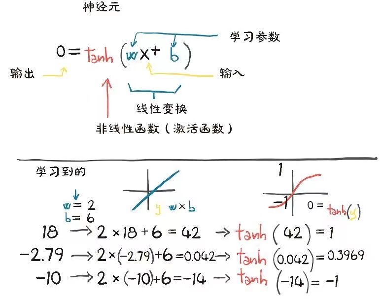
从数学上讲，我们可以写成 o=f(wx+b)o =f(wx+b)o=f(wx+b)，其中 xxx 是输入， www是权重或比例因子，bbb是偏置或偏移量，fff 是激活函数，设为双曲正切，这里是 tanhtanhtanh函数。 通常，xxx 和 ooo 可以是单个标量或矩阵，而 bbb 是标量或向量。

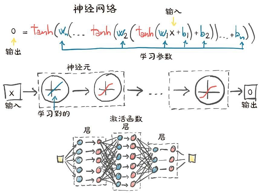
多层网络

前一层神经元的输出被用作后一层神经元的输入

完整代码

我们刚从一个地方旅游回来，带回了一个别致的壁挂式模拟温度计，但是不显示单位。

利用卷积网络，迭代地调整它的权重，直到误差的度量足够低，最终能够以我们选择的单位来解释新的刻度值

import torch
import torch.optim as optim
import torch.nn as nn
from collections import OrderedDict

t_c = [0.5,  14.0, 15.0, 28.0, 11.0,  8.0,  3.0, -4.0,  6.0, 13.0, 21.0]
t_u = [35.7, 55.9, 58.2, 81.9, 56.3, 48.9, 33.9, 21.8, 48.4, 60.4, 68.4]
t_c = torch.tensor(t_c).unsqueeze(1) # <1> 转置
t_u = torch.tensor(t_u).unsqueeze(1) # <1> 转置

### 按训练、验证 进行分割数据
n_samples = t_u.shape[0]
n_val = int(0.2 * n_samples)

shuffled_indices = torch.randperm(n_samples)

train_indices = shuffled_indices[:-n_val]
val_indices = shuffled_indices[-n_val:]

t_u_train = t_u[train_indices]
t_c_train = t_c[train_indices]

t_u_val = t_u[val_indices]
t_c_val = t_c[val_indices]

t_un_train = 0.1 * t_u_train  # 数据归一化
t_un_val = 0.1 * t_u_val      # 数据归一化

seq_model = nn.Sequential(OrderedDict([
    ('hidden_linear', nn.Linear(1, 8)),
    ('hidden_activation', nn.Tanh()),
    ('output_linear', nn.Linear(8, 1))
]))

optimizer = optim.SGD(seq_model.parameters(), lr=1e-3) # <1>

def training_loop(n_epochs, optimizer, model, loss_fn, t_u_train, t_u_val,
                  t_c_train, t_c_val):
    for epoch in range(1, n_epochs + 1):
        t_p_train = model(t_u_train) # <1>
        loss_train = loss_fn(t_p_train, t_c_train)

        t_p_val = model(t_u_val) # <1>
        loss_val = loss_fn(t_p_val, t_c_val)
        
        optimizer.zero_grad()
        loss_train.backward() # <2>
        optimizer.step()

        if epoch == 1 or epoch % 1000 == 0:
            print(f"Epoch {epoch}, Training loss {loss_train.item():.4f},"
                  f" Validation loss {loss_val.item():.4f}")


training_loop(
    n_epochs = 5000, 
    optimizer = optimizer,
    model = seq_model,
    loss_fn = nn.MSELoss(),
    t_u_train = t_un_train,
    t_u_val = t_un_val, 
    t_c_train = t_c_train,
    t_c_val = t_c_val)
    
print('output', seq_model(t_un_val))
print('answer', t_c_val)
print('hidden', seq_model.hidden_linear.weight.grad)

Epoch 1, Training loss 197.4816, Validation loss 112.5018
Epoch 1000, Training loss 5.0292, Validation loss 6.4672
Epoch 2000, Training loss 3.6761, Validation loss 3.5783
Epoch 3000, Training loss 1.8501, Validation loss 4.1298
Epoch 4000, Training loss 1.3914, Validation loss 5.0082
Epoch 5000, Training loss 1.3010, Validation loss 5.7680
output tensor([[13.2498],
        [ 0.0773]], grad_fn=<AddmmBackward0>)
answer tensor([[15.],
        [ 3.]])
hidden tensor([[-0.1139],
        [ 0.1778],
        [ 0.1690],
        [-0.0255],
        [-0.1855],
        [-0.0152],
        [ 0.0058],
        [ 0.1020]])

torch.nn.Linear()

torch.nn.Linear(in_features, out_features, bias=True) 是 PyTorch 中实现全连接（线性/仿射）变换的层，对输入张量最后一维执行操作：

output=xWT+biasoutput = x W ^T + biasoutput=xWT+bias

其中，W是形状为(out_features, in_features)的权重矩阵 ，b是长度为out_features的偏置向量。

‌in_features‌：输入张量最后一维的大小（必填）；

‌out_features‌：输出张量最后一维的大小（必填）；

‌bias‌：是否含可学习偏置，默认 True；

linear_model = torch.nn.Linear(1, 1)
print(linear_model.parameters())
list(linear_model.parameters())

<generator object Module.parameters at 0x119a74ba0>
[Parameter containing:
 tensor([[0.3980]], requires_grad=True),
 Parameter containing:
 tensor([-0.6486], requires_grad=True)]

torch.nn.Sequential()

‌torch.nn.Sequential() 是 PyTorch 中用于快速搭建顺序神经网络的容器模块‌，它能把多个网络层按顺序打包成一个整体，数据会自动从第一层流到最后一层，无需手动写前向传播代码

seq_model = torch.nn.Sequential(
                torch.nn.Linear(1,8),
                torch.nn.Tanh(),
                torch.nn.Linear(8,1))
print(seq_model)

for name,param in seq_model.named_parameters():
    print(name, param.shape)

Sequential(
  (0): Linear(in_features=1, out_features=8, bias=True)
  (1): Tanh()
  (2): Linear(in_features=8, out_features=1, bias=True)
)
0.weight torch.Size([8, 1])
0.bias torch.Size([8])
2.weight torch.Size([1, 8])
2.bias torch.Size([1])

collections.OrderedDict()

‌用 OrderedDict命名‌：给每层起个名字，后续调试和修改更方便，推荐用于稍复杂的模型

from collections import OrderedDict
seq_model = nn.Sequential(OrderedDict([
    ('hidden_linear', nn.Linear(1, 8)),
    ('hidden_activation', nn.Tanh()),
    ('output_linear', nn.Linear(8, 1))
]))
print(seq_model)

for name,param in seq_model.named_parameters():
    print(name, param.shape)

Sequential(
  (hidden_linear): Linear(in_features=1, out_features=8, bias=True)
  (hidden_activation): Tanh()
  (output_linear): Linear(in_features=8, out_features=1, bias=True)
)
hidden_linear.weight torch.Size([8, 1])
hidden_linear.bias torch.Size([8])
output_linear.weight torch.Size([1, 8])
output_linear.bias torch.Size([1])

torch.nn.MSELoss() 均方误差

torch.nn.MSELoss 是 PyTorch 中的均方误差损失函数。

它计算预测值与目标值之间差值的平方均值，常用于回归任务。

函数定义

torch.nn.MSELoss(reduction='mean')

参数说明：

reduction (str): 损失聚合方式。可选 'mean'、'sum'、'none'。默认为 'mean'。

数学原理

MSE 损失公式：

MSE=(1/n)∗∑(ypred−ytrue)2MSE = (1/n) *\sum(y_{pred} - y_{true})^2MSE=(1/n)∗∑(ypred−ytrue)2

模型输出拟合可视化

from matplotlib import pyplot as plt
from matplotlib import font_manager
# macOS 中文字体路径
myfont = font_manager.FontProperties(fname="/System/Library/Fonts/Supplemental/Arial Unicode.ttf")

t_range = torch.arange(20., 90.).unsqueeze(1)

fig = plt.figure(dpi=600)
plt.xlabel('温度---摄氏度',fontproperties=myfont)
plt.ylabel('测量值',fontproperties=myfont)
plt.plot(t_u.numpy(), t_c.numpy(), 'o')
plt.plot(t_range.numpy(), seq_model(0.1 * t_range).detach().numpy(), 'c-')
plt.plot(t_u.numpy(), seq_model(0.1 * t_u).detach().numpy(), 'kx')
plt.savefig("神经网络-拟合线.png")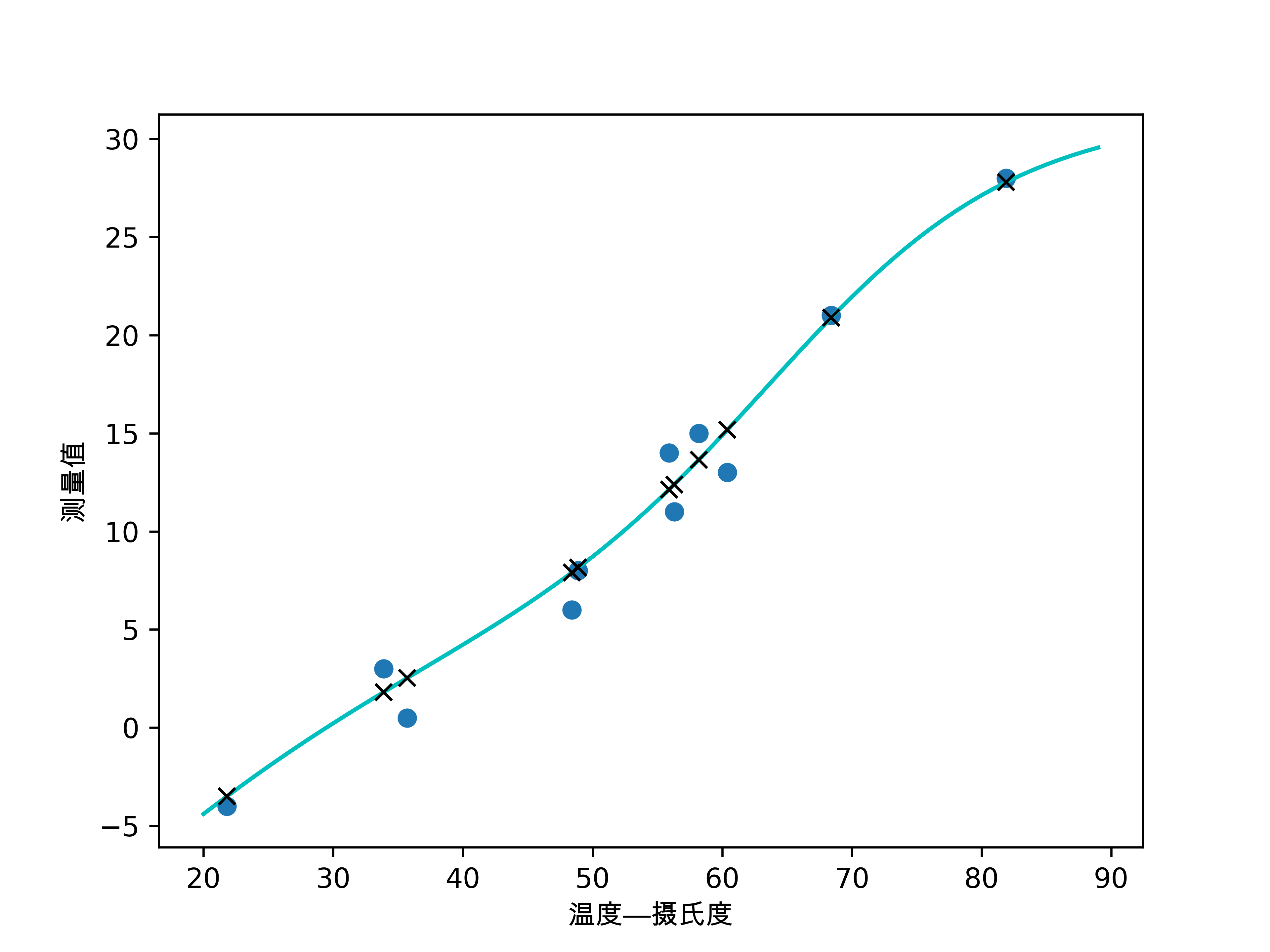

输入数据（用圆圈表示）和 模型输出（用X表示）