从零写一个 Attention Is All You Need

Transformer 源码深度剖析

1. 开始

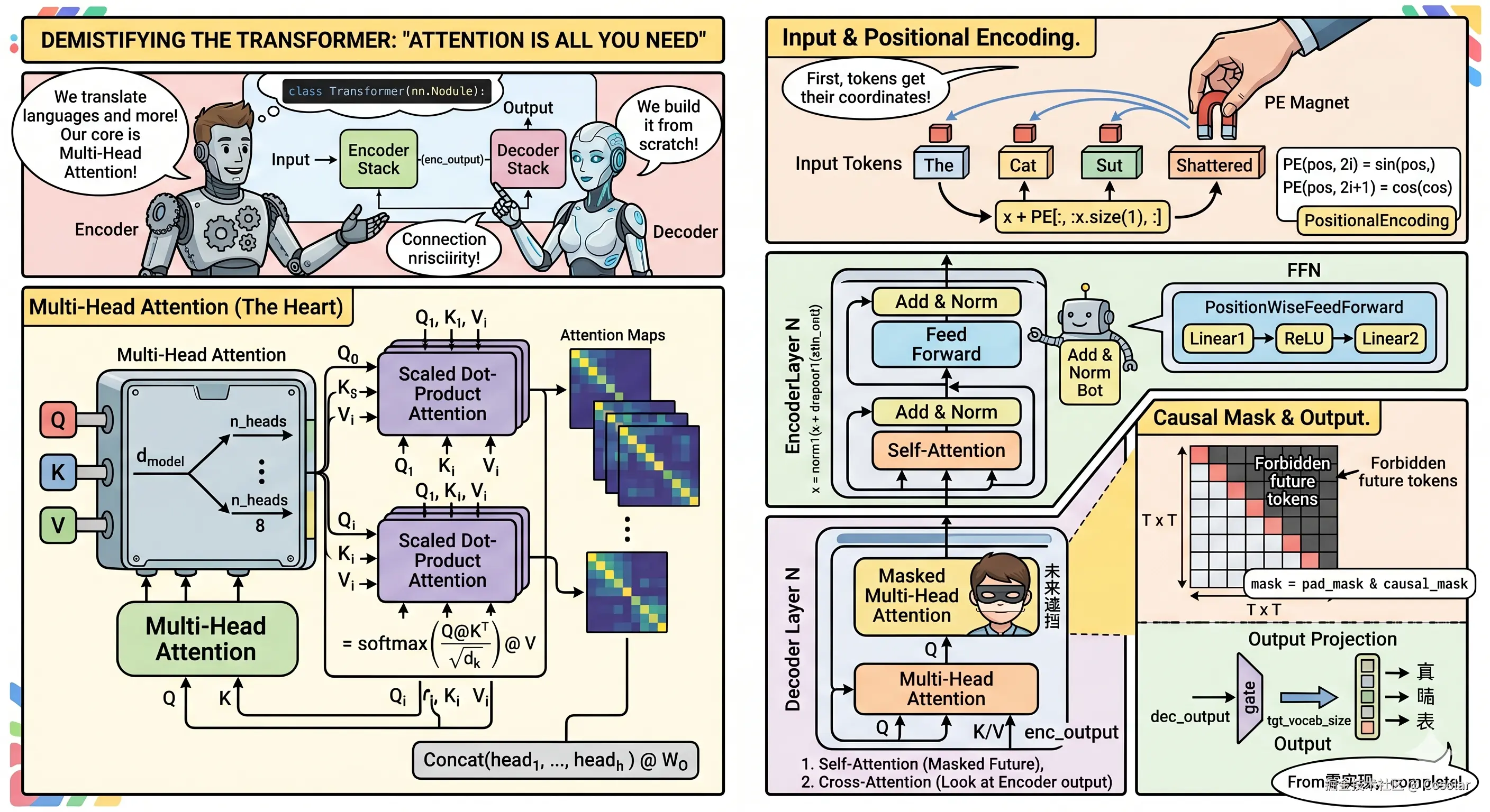
2017 年，Google 研究团队发表论文 《Attention Is All You Need》，提出 Transformer 架构。它彻底弃用了 RNN/LSTM 递归结构，完全依赖 Attention 机制捕获语义关系，开启了 GPT、BERT、LLaMA 等大模型的时代。

本文通过一份干净的从零实现代码（约 350 行，纯 PyTorch），逐层剖析 Transformer 的每一个组件。代码可直接运行，适合学习者理解原理、调试和二次开发。

组件一览

组件	功能	复杂度
Scaled Dot-Product Attention	Q/K/V 相似度计算与聚合	O(n·dₖ)
Multi-Head Attention	多个表示空间并行注意力	O(n·d_model)
Position-wise FFN	每个位置非线性变换	O(d_model·d_ff)
Positional Encoding	引入位置信息	O(max_len·d_model)
Layer Norm	维度规范化	O(d_model)
Encoder Layer	自注意力 + FFN	O(n²·d_model)
Decoder Layer	带掩码 + 交叉注意力	O(n²·d_model)

---

2. Scaled Dot-Product Attention

公式与直观

Scaled Dot-Product Attention 是 Transformer 的核心计算单元。其本质是 "查询"（Query）与 "键"（Key）的相似度来对 "值"（Value）进行加权聚合：

$Attention(Q,K,V)=softmax\; (\; QK\top \; dk\; )\; V\backslash text\{Attention\}(Q,\; K,\; V)\; =\; \backslash text\{softmax\}\backslash left(\backslash frac\{QK^\backslash top\}\{\backslash sqrt\{d\_k\}\}\backslash right)V$ Attention(Q,K,V)=softmax(dk QK⊤)V

为什么要除以 $dk\; \backslash sqrt\{d\_k\}$ dk ？ 当 $dk\; d\_k$ dk 较大时，点积的模值随维度增加而增大，将 softmax 推向极端区域（梯度消失）。缩放后方差保持稳定，训练更稳定。

代码解析

class ScaledDotProductAttention(nn.Module):
    """
    Attention(Q, K, V) = softmax(Q @ K^T / sqrt(d_k)) @ V
    """
    def __init__(self, dropout: float = 0.1):
        super().__init__()
        self.dropout = nn.Dropout(dropout)

    def forward(self, Q, K, V, mask=None):
        d_k = Q.size(-1)
        scores = torch.matmul(Q, K.transpose(-2, -1)) / math.sqrt(d_k)

        if mask is not None:
            scores = scores.masked_fill(mask == 0, float('-inf'))

        attn_weights = F.softmax(scores, dim=-1)
        attn_weights = self.dropout(attn_weights)
        output = torch.matmul(attn_weights, V)
        return output, attn_weights

key takeaways:

• masked_fill 将 padding 位置赋值为 -inf，softmax 后权重为 0，不影响输出
• Attention 权重计算后再 dropout，是重要的正则化手段
• 返回 attn_weights 主要用于可视化和调试

复杂度来自 $QK\top QK^\backslash top$ QK⊤ 矩阵乘法，为 $O(n2\cdot dk)\; O(n^2\; \backslash cdot\; d\_k)$ O(n2⋅dk)，其中 $nn$ n 为序列长度。这是 Transformer 的性能瓶颈。

---

3. Multi-Head Attention

从单头到多头

单头注意力只能关注一个表示空间。Multi-Head Attention 将 Q/K/V 分别投影到 $hh$ h 个不同的表示空间，在每个子空间独立计算注意力，最后拼接并投影回 $dmodel\; d\_\{model\}$ dmodel 维度。

$MultiHead(Q,K,V)=Concat(head1,...,headh)WO\backslash text\{MultiHead\}(Q,K,V)\; =\; \backslash text\{Concat\}(\backslash text\{head\}\_1,\; ...,\; \backslash text\{head\}\_h)W\_O$ MultiHead(Q,K,V)=Concat(head1,...,headh)WO

代码中的关键设计决策：先投影再拆头 。定义 $hh$ h 个独立线性层在数学上等价，但只需 4 个线性层，而非 $3h3h$ 3h 个，更高效。

代码解析

class MultiHeadAttention(nn.Module):
    """
    MultiHead(Q, K, V) = Concat(head_1, ..., head_h) @ W_O
    其中 head_i = Attention(Q @ W_Q_i, K @ W_K_i, V @ W_V_i)
    """
    def __init__(self, d_model: int, n_heads: int, dropout: float = 0.1):
        super().__init__()
        assert d_model % n_heads == 0, "d_model 必须能被 n_heads 整除"

        self.d_model = d_model
        self.n_heads = n_heads
        self.d_k = d_model // n_heads

        self.W_Q = nn.Linear(d_model, d_model, bias=False)
        self.W_K = nn.Linear(d_model, d_model, bias=False)
        self.W_V = nn.Linear(d_model, d_model, bias=False)
        self.W_O = nn.Linear(d_model, d_model, bias=False)

        self.attention = ScaledDotProductAttention(dropout)

    def forward(self, Q, K, V, mask=None):
        batch_size = Q.size(0)

        # 1) 线性投影 → (batch, seq_len, d_model)
        Q = self.W_Q(Q)
        K = self.W_K(K)
        V = self.W_V(V)

        # 2) 拆成多头 → (batch, n_heads, seq_len, d_k)
        Q = Q.view(batch_size, -1, self.n_heads, self.d_k).transpose(1, 2)
        K = K.view(batch_size, -1, self.n_heads, self.d_k).transpose(1, 2)
        V = V.view(batch_size, -1, self.n_heads, self.d_k).transpose(1, 2)

        # 3) Scaled Dot-Product Attention
        attn_output, attn_weights = self.attention(Q, K, V, mask)

        # 4) 拼接多头 → (batch, seq_len, d_model)
        attn_output = attn_output.transpose(1, 2).contiguous().view(
            batch_size, -1, self.d_model
        )

        # 5) 最终线性投影
        output = self.W_O(attn_output)
        return output

key takeaways:

• d_model % n_heads == 0：确保每个 head 分到整数维度
• view + transpose：先拆开维度再转置，像"再排片"一样得到 head 维度在第一维
• .contiguous()：transpose 只是视图，内存布局未变，contiguous 保证后续 view 不报错
• W_O：拼接后的最终投影，融合多头信息回 d_model

注意代码中的 mask 处理：mask 为 (batch, 1, 1, seq_len) 格式，可直接与 scores (batch, n_heads, seq_len, seq_len) 广播，无需额外 unsqueeze。

---

4. Position-wise Feed-Forward Network

非线性变换与容量

每个位置的表示在经过注意力层后，还要经过一个两层的全连接网络。这个 FFN 是 position-wise 的------对序列中每个位置独立应用相同的参数，相当于 kernel size = 1 的卷积。

$FFN(x)=ReLU(xW1+b1)W2+b2\backslash text\{FFN\}(x)\; =\; \backslash text\{ReLU\}(xW\_1\; +\; b\_1)W\_2\; +\; b\_2$ FFN(x)=ReLU(xW1+b1)W2+b2

代码解析

class PositionWiseFeedForward(nn.Module):
    """
    FFN(x) = ReLU(x @ W_1 + b_1) @ W_2 + b_2
    内部维度从 d_model → d_ff → d_model
    """
    def __init__(self, d_model: int, d_ff: int, dropout: float = 0.1):
        super().__init__()
        self.linear1 = nn.Linear(d_model, d_ff)
        self.linear2 = nn.Linear(d_ff, d_model)
        self.dropout = nn.Dropout(dropout)

    def forward(self, x):
        return self.linear2(self.dropout(F.relu(self.linear1(x))))

key takeaways:

• 内部维度 d_ff 通常比 d_model 大得多（论文中 512 → 2048），提供了非线性变换的容量
• dropout 放在 ReLU 之后、第二次线性投影之前，是流行的做法
• 原始论文用 ReLU，后来的 GPT 等工作更多用 GELU

为什么两层？ 论文实验表明一层表达能力不足，三层以上收益微乎其微。两层是性能与资源的最优解。

---

5. Positional Encoding

为序列引入位置信息

Self-Attention 是 "位置不敏感" 的------对序列的任意 permutation，输出都是相同的。为了引入位置信息，原始论文使用正余弦编码（Sinusoidal Positional Encoding）：

$PE(pos,2i)=sin\; (\; pos10000\; 2i/\; dmodel\; )\; \backslash text\{PE\}(pos,\; 2i)\; =\; \backslash sin\backslash left(\backslash frac\{pos\}\{10000^\{2i/d\_\{model\}\}\}\backslash right)$ PE(pos,2i)=sin(100002i/dmodelpos)

$PE(pos,2i+1)=cos\; (\; pos10000\; 2i/\; dmodel\; )\; \backslash text\{PE\}(pos,\; 2i+1)\; =\; \backslash cos\backslash left(\backslash frac\{pos\}\{10000^\{2i/d\_\{model\}\}\}\backslash right)$ PE(pos,2i+1)=cos(100002i/dmodelpos)

为什么用正余弦而不用可学习的位置嵌入？

1. 可以处理比训练时更长的序列（外推）
2. 不需要参数，减少内存
3. 相对位置信息可以通过线性变换表达（因为 $sin(\alpha +\Delta )=sin\alpha \cdot cos\Delta +cos\alpha \cdot sin\Delta \backslash sin(\backslash alpha+\backslash Delta)\; =\; \backslash sin\backslash alpha\; \backslash cdot\; \backslash cos\backslash Delta\; +\; \backslash cos\backslash alpha\; \backslash cdot\; \backslash sin\backslash Delta$ sin(α+Δ)=sinα⋅cosΔ+cosα⋅sinΔ------存在线性关系）

代码解析

class PositionalEncoding(nn.Module):
    """
    PE(pos, 2i)   = sin(pos / 10000^(2i/d_model))
    PE(pos, 2i+1) = cos(pos / 10000^(2i/d_model))
    """
    def __init__(self, d_model: int, max_len: int = 5000, dropout: float = 0.1):
        super().__init__()
        self.dropout = nn.Dropout(dropout)

        pe = torch.zeros(max_len, d_model)
        position = torch.arange(0, max_len, dtype=torch.float).unsqueeze(1)
        div_term = torch.exp(
            torch.arange(0, d_model, 2).float() * (-math.log(10000.0) / d_model)
        )

        pe[:, 0::2] = torch.sin(position * div_term)  # 偶数维度
        pe[:, 1::2] = torch.cos(position * div_term)  # 奇数维度

        pe = pe.unsqueeze(0)
        self.register_buffer('pe', pe)

    def forward(self, x):
        x = x + self.pe[:, :x.size(1), :]
        return self.dropout(x)

key takeaways:

• div_term 采用指数形式而非直接计算 $10000\; 2i/\; dmodel\; 10000^\{2i/d\_\{model\}\}$ 100002i/dmodel，是为了数值稳定性
• register_buffer 让 pe 随模型移动到 CPU/GPU，但不会作为参数被优化
• forward 中直接相加（broadcast），是最经典的位置嵌入方式

---

6. Layer Normalization

维度规范化

Layer Normalization 是对每个样本的所有维度做变换：减去均值、除以标准差，再做可学习的线性变换。与 Batch Norm 不同，LN 不依赖 batch 大小，在处理变长序列时更稳定。

$LayerNorm(x)=\gamma \cdot \; x-\mu \; \sigma 2+ϵ\; +\beta \backslash text\{LayerNorm\}(x)\; =\; \backslash gamma\; \backslash cdot\; \backslash frac\{x\; -\; \backslash mu\}\{\backslash sqrt\{\backslash sigma^2\; +\; \backslash epsilon\}\}\; +\; \backslash beta$ LayerNorm(x)=γ⋅σ2+ϵ x−μ+β

代码解析

class LayerNorm(nn.Module):
    """
    LayerNorm(x) = gamma * (x - mean) / sqrt(var + eps) + beta
    手写版，方便理解；实际可直接用 nn.LayerNorm
    """
    def __init__(self, d_model: int, eps: float = 1e-6):
        super().__init__()
        self.gamma = nn.Parameter(torch.ones(d_model))
        self.beta = nn.Parameter(torch.zeros(d_model))
        self.eps = eps

    def forward(self, x):
        mean = x.mean(dim=-1, keepdim=True)
        std = x.std(dim=-1, keepdim=True, unbiased=False)
        return self.gamma * (x - mean) / (std + self.eps) + self.beta

key takeaways:

• 手写版方便理解，生产代码可直接用 nn.LayerNorm
• unbiased=False：使用样本标准差而非无偏估计，与原始论文一致
• eps 防止除零，经典取值 1e-6

---

7. Encoder Layer

网络中的网络单元

Encoder 层是 Transformer 的基本构建块。每层包含两个子层：多头自注意力 和 FFN ，每个子层后跟一个残差连接 + 层规范化。

x → MultiHead Self-Attention → Add & Norm → FFN → Add & Norm

代码解析

class EncoderLayer(nn.Module):
    """
    一个 Encoder 层：
      x → MultiHead Self-Attention → Add & Norm → FFN → Add & Norm
    """
    def __init__(self, d_model: int, n_heads: int, d_ff: int,
                 dropout: float = 0.1):
        super().__init__()
        self.self_attn = MultiHeadAttention(d_model, n_heads, dropout)
        self.ffn = PositionWiseFeedForward(d_model, d_ff, dropout)
        self.norm1 = LayerNorm(d_model)
        self.norm2 = LayerNorm(d_model)
        self.dropout1 = nn.Dropout(dropout)
        self.dropout2 = nn.Dropout(dropout)

    def forward(self, x, mask=None):
        # Self-Attention + Add & Norm
        attn_output = self.self_attn(x, x, x, mask)
        x = x + self.dropout1(attn_output)
        x = self.norm1(x)

        # FFN + Add & Norm
        ffn_output = self.ffn(x)
        x = x + self.dropout2(ffn_output)
        x = self.norm2(x)

        return x

key takeaways:

• 残差连接 （ $x+sublayer(x)x\; +\; \backslash text\{sublayer\}(x)$ x+sublayer(x)）解决深层网络的梯度消失问题------梯度可以直接流过 shortcut 回传
• 这是 Post-LN 模式：先残差再规范化，与原始论文一致
• self_attn 的三个参数都是 $xx$ x，表示 "自注意力"------Q、K、V 来自同一个序列

---

8. Decoder Layer

带掩码的自注意力与交叉注意力

Decoder 层比 Encoder 多了一个子层：Cross-Attention （以 Encoder 输出为 K/V，Decoder 输入为 Q）。同时自注意力层要用下三角 mask 掩码后续位置，防止泄露未来信息。

x → Masked Self-Attention → Add & Norm → Cross-Attention → Add & Norm → FFN → Add & Norm

代码解析

class DecoderLayer(nn.Module):
    def __init__(self, d_model: int, n_heads: int, d_ff: int,
                 dropout: float = 0.1):
        super().__init__()
        self.self_attn = MultiHeadAttention(d_model, n_heads, dropout)
        self.cross_attn = MultiHeadAttention(d_model, n_heads, dropout)
        self.ffn = PositionWiseFeedForward(d_model, d_ff, dropout)

        self.norm1 = LayerNorm(d_model)
        self.norm2 = LayerNorm(d_model)
        self.norm3 = LayerNorm(d_model)

        self.dropout1 = nn.Dropout(dropout)
        self.dropout2 = nn.Dropout(dropout)
        self.dropout3 = nn.Dropout(dropout)

    def forward(self, x, enc_output, src_mask=None, tgt_mask=None):
        # Self-Attention（带 look-ahead mask）
        attn_output = self.self_attn(x, x, x, tgt_mask)
        x = x + self.dropout1(attn_output)
        x = self.norm1(x)

        # Cross-Attention: Q 来自 Decoder, K/V 来自 Encoder
        attn_output = self.cross_attn(x, enc_output, enc_output, src_mask)
        x = x + self.dropout2(attn_output)
        x = self.norm2(x)

        # FFN
        ffn_output = self.ffn(x)
        x = x + self.dropout3(ffn_output)
        x = self.norm3(x)

        return x

key takeaways:

• Self-Attention 用 tgt_mask（下三角）掩码后续位置，Cross-Attention 用 src_mask（过滤 encoder padding）
• Cross-Attention 的 K/V 来自 Encoder，Q 来自 Decoder------这是"引导"机制，Decoder 每一步都能"看到"输入序列的全部信息
• Decoder 有 3 个残差连接 + 3 个 LayerNorm

---

9. 完整 Transformer

拼装成网络

最后，将 N 层 Encoder 和 N 层 Decoder 堆叠起来，再加上嵌入层、位置编码和最终分类头，就是完整的 Transformer。

src → Embedding → Positional Encoding → N × EncoderLayer
                                              ↓
tgt → Embedding → Positional Encoding → N × DecoderLayer → Linear → output

代码解析

class Transformer(nn.Module):
    def __init__(self, src_vocab, tgt_vocab, d_model=512,
                 n_heads=8, d_ff=2048, n_layers=6,
                 dropout=0.1, max_len=5000):
        super().__init__()
        self.encoder_embed = nn.Embedding(src_vocab, d_model)
        self.decoder_embed = nn.Embedding(tgt_vocab, d_model)
        self.pos_encoding = PositionalEncoding(d_model, max_len, dropout)

        self.encoder_layers = nn.ModuleList([
            EncoderLayer(d_model, n_heads, d_ff, dropout)
            for _ in range(n_layers)
        ])
        self.decoder_layers = nn.ModuleList([
            DecoderLayer(d_model, n_heads, d_ff, dropout)
            for _ in range(n_layers)
        ])

        self.fc_out = nn.Linear(d_model, tgt_vocab)

    def forward(self, src, tgt, src_mask=None, tgt_mask=None):
        # Encoder
        src_emb = self.pos_encoding(self.encoder_embed(src))
        for layer in self.encoder_layers:
            src_emb = layer(src_emb, src_mask)

        # Decoder
        tgt_emb = self.pos_encoding(self.decoder_embed(tgt))
        for layer in self.decoder_layers:
            tgt_emb = layer(tgt_emb, src_emb, src_mask, tgt_mask)

        return self.fc_out(tgt_emb)

key takeaways:

• nn.ModuleList 保证每层的参数都被正确登记
• Encoder/Decoder 各自有独立的嵌入层和位置编码
• fc_out 将 d_model 投影到词表大小，用于生成下一个 token 的概率分布

---

10. 总结

这份从零实现覆盖了 Transformer 的所有核心组件。从 Scaled Dot-Product Attention 到完整的 Encoder-Decoder 架构，每一行代码都有明确的意义和设计思考。

了解这些基础组件后，再去看 GPT 系列的只用 Decoder 、BERT 系列的只用 Encoder，以及 LLaMA 等现代变体时，就能很快把握住它们的设计决策。