Delaunay 拓扑图割法一种特征抽稀算法

这个算法利用点与点之间的连线关系（拓扑网络）来剔除内部杂波。内部干扰点的特征是：它们与周围点的连接是短小、杂乱、蜘蛛网状的；而外轮廓点的连接是长距离、大跨度、形成闭环的。

核心逻辑：

我们将点连接成网，然后用 Scale 参数作为"剪刀"，剪断太短的线（局部杂波），保留能形成大环的线（外轮廓）。

算法步骤：

1. 建网：对所有特征点进行 Delaunay 三角剖分，得到一个拓扑网络。
   计算边长：计算网络中所有边的长度。
   拓扑剪枝（核心）：
   遍历所有边，如果边长L>Scale，保留该边；如果 L<Scale，剪断该边。
   注意：内部杂乱点之间的距离通常很短，它们的连接会被全部剪断，变成"孤岛"。
2. 连通域分析：
   剪枝后，寻找最大连通子图（或者形成闭环的子图）。外轮廓点因为跨距大，往往能连成一个大环。
   剔除掉度数为0的孤立点（即内部被剪断的杂波点）。
   骨架重采样（可选）：如果抽稀后外轮廓点仍然太密，可以在保留的大环上进行等距采样。

打个比方：

这就像修剪灌木丛。Scale 是剪刀的尺寸。外轮廓是粗壮的藤蔓（间距大，剪不断），内部杂草是细小的枝桠（间距小，一剪子下去全断）。剪完之后，抖一抖（剔除孤立点），杂草掉光，只剩藤蔓骨架。

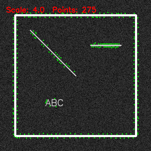
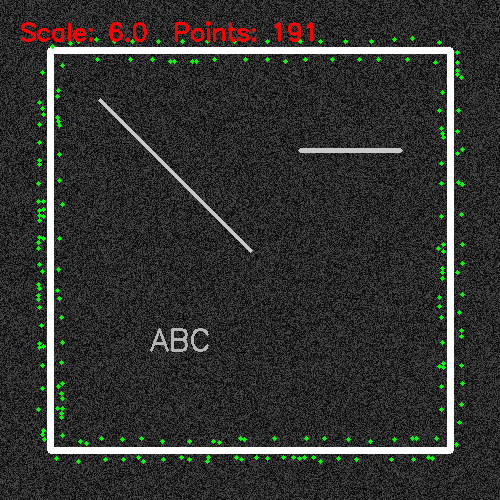
效果图

代码

import cv2
import numpy as np
from scipy.spatial import Delaunay
from collections import deque

def smart_feature_thinning_v3(img, scale=1.0, base_radius=2, contour_protect_radius=3, grad_threshold=30):
    """
    V3: Delaunay 拓扑图割法 (彻底抛弃Canny，纯粹基于点空间关系的拓扑抽稀)
    
    参数:
        img: 输入灰度图
        scale: 抽稀尺度 (1.0 - 10.0)，控制拓扑剪刀的阈值
        base_radius: 内部点基础抑制半径
        contour_protect_radius: 骨架保护半径
        grad_threshold: 基础梯度阈值
    """
    # 1. 尺度空间高斯模糊 (保留，依然非常有助于源头压制高频杂波)
    sigma = max(0.1, scale * 1.5)
    ksize = int(sigma * 6) | 1  
    blurred = cv2.GaussianBlur(img, (ksize, ksize), sigmaX=sigma, sigmaY=sigma)

    # 2. 计算梯度
    grad_x = cv2.Sobel(blurred, cv2.CV_32F, 1, 0, ksize=3)
    grad_y = cv2.Sobel(blurred, cv2.CV_32F, 0, 1, ksize=3)
    grad_mag = np.sqrt(grad_x**2 + grad_y**2)
    
    # 3. 提取候选点 (局部极大值)
    mask = (grad_mag > grad_threshold)
    local_max_mask = np.zeros_like(mask)
    for i in range(1, img.shape[0]-1):
        for j in range(1, img.shape[1]-1):
            region = grad_mag[i-1:i+2, j-1:j+2]
            if grad_mag[i, j] == np.max(region) and mask[i, j]:
                local_max_mask[i, j] = True
                
    ys, xs = np.where(local_max_mask)
    scores = grad_mag[ys, xs]
    
    # 按照得分从高到低排序
    order = np.argsort(-scores)
    xs, ys, scores = xs[order], ys[order], scores[order]
    
    # 点数太少无法构建拓扑，直接返回
    if len(xs) < 3:
        return list(zip(xs, ys))

    # ================= 【核心重写：Delaunay 拓扑图割】 =================
    points = np.column_stack((xs, ys))
    
    # 4. 构建 Delaunay 三角剖分
    tri = Delaunay(points)
    
    # 提取所有唯一的边
    edges = set()
    for simplex in tri.simplices:
        edges.add(tuple(sorted((simplex[0], simplex[1]))))
        edges.add(tuple(sorted((simplex[1], simplex[2]))))
        edges.add(tuple(sorted((simplex[0], simplex[2]))))
        
    # 5. 拓扑剪枝 (图割)
    # Scale 越大，短边阈值越长，内部杂波网状连接被剪得越碎
    min_edge_len = scale * 2.0  
    # 跨越图像空洞的内部对角线通常很长，也要剪断，防止内部点连到外轮廓上
    max_edge_len = min(img.shape[0], img.shape[1]) * 0.15  
    
    adj = {i: [] for i in range(len(points))}
    for i, j in edges:
        dist = np.linalg.norm(points[i] - points[j])
        # 只保留长度适中的 "结构边" (骨架边)
        if min_edge_len <= dist <= max_edge_len:
            adj[i].append(j)
            adj[j].append(i)
            
    # 6. 连通域分析 (BFS寻岛)
    # 剪枝后，内部杂波变成孤立点或极小簇，外轮廓依然是大簇
    visited = [False] * len(points)
    is_structure = [False] * len(points)
    min_cluster_size = 3  # 至少3个点相连，才算拓扑骨架/外轮廓
    
    for i in range(len(points)):
        if not visited[i]:
            cluster = []
            queue = deque([i])
            visited[i] = True
            while queue:
                curr = queue.popleft()
                cluster.append(curr)
                for neighbor in adj[curr]:
                    if not visited[neighbor]:
                        visited[neighbor] = True
                        queue.append(neighbor)
            
            # 大簇保留，小簇和孤立点标记为非结构(杂波)
            if len(cluster) >= min_cluster_size:
                for idx in cluster:
                    is_structure[idx] = True
    # ==================================================================

    # 7. 拓扑感知非对称 NMS
    keep_points = []
    internal_radius = base_radius + int(scale * 2.5) 
    
    suppressed = np.zeros(img.shape[:2], dtype=bool)
    
    for i in range(len(xs)):
        x, y = xs[i], ys[i]
        
        if suppressed[y, x]:
            continue
            
        keep_points.append((x, y))
        
        # 判断身份：由 Delaunay 拓扑图割决定
        if is_structure[i]:
            r = contour_protect_radius  # 属于拓扑骨架：小半径保护
        else:
            r = internal_radius          # 属于孤立杂波：大范围清洗
            
        # 标记抑制区域
        y_top = max(0, y - r)
        y_bot = min(img.shape[0], y + r + 1)
        x_left = max(0, x - r)
        x_right = min(img.shape[1], x + r + 1)
        suppressed[y_top:y_bot, x_left:x_right] = True
        
    return keep_points


# ================= 测试与可视化代码 =================

def on_trackbar(val):
    scale_val = val / 10.0
    if scale_val < 0.1: scale_val = 0.1
    
    points = smart_feature_thinning_v3(img_gray, scale=scale_val, 
                                       base_radius=2, contour_protect_radius=3, 
                                       grad_threshold=30)
    
    display = img_color.copy()
    for (x, y) in points:
        cv2.circle(display, (x, y), 2, (0, 255, 0), -1)
        
    cv2.putText(display, f"Scale: {scale_val:.1f}  Points: {len(points)}", 
                (20, 40), cv2.FONT_HERSHEY_SIMPLEX, 0.8, (0, 0, 255), 2)
    
    cv2.imshow("V3 Delaunay Topology Cut Thinning", display)

# 生成挑战性测试图
img_color = np.zeros((500, 500, 3), dtype=np.uint8)
img_gray = np.zeros((500, 500), dtype=np.uint8)

cv2.rectangle(img_gray, (50, 50), (450, 450), 255, 5)
cv2.line(img_gray, (100, 100), (250, 250), 200, 3)
cv2.line(img_gray, (300, 150), (400, 150), 200, 3)
cv2.putText(img_gray, "ABC", (150, 350), cv2.FONT_HERSHEY_SIMPLEX, 1, 180, 2)
noise = np.random.randint(0, 80, (500, 500), dtype=np.uint8)
img_gray = np.maximum(img_gray, noise)

# 如果有真实图片，取消下面这行注释
# img_gray = cv2.imread("model.jpg", cv2.IMREAD_GRAYSCALE)
# img_color = cv2.cvtColor(img_gray, cv2.COLOR_GRAY2BGR)

if len(img_gray.shape) == 2:
    img_color = cv2.cvtColor(img_gray, cv2.COLOR_GRAY2BGR)

cv2.namedWindow("V3 Delaunay Topology Cut Thinning")
cv2.createTrackbar("Scale (1-100)", "V3 Delaunay Topology Cut Thinning", 10, 100, on_trackbar)

on_trackbar(10)
cv2.waitKey(0)
cv2.destroyAllWindows()