【ch04】Implementing-a-GPT-model-from-scratch-to-generate-text

零、前言

这一章作者带着手搓了一下GPT 2的architecture，架构还是比价清晰易懂的。

本章代码：ch04

一、Implementing a GPT model

1.1 Coding a LLM architecture

像**GPT(generative pretrained transformer)**这样的LLM，都是大而深的神经网络架构，使得生成文本时一次生成一个单词。

虽然模型很庞大，但是架构本身却没有想象中的那么复杂。

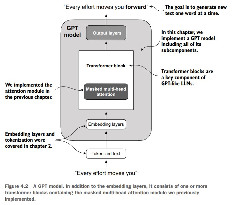
本章将会实现GPT-2 small的架构，参数量为124M。

在深度学习，或者是LLM领域提到的参数量，往往是指模型的可训练权重。这些权重本质上是模型训练过程中为了最小化loss时的内部变量。

比如一个神经网络层用一个2048*2048的矩阵表示权重，那么这个层的参数量就是2048 * 2048 = 4,194,304。

作者选择实现GPT-2是因为 Open AI开源了GPT-2的预训练权重，在第六章作者会加载这些权重。

GPT-3的模型架构和GPT-2基本类似，只不过从GPT-2XL的1.5B权重上升到了175B。

GPT-3的训练需要更大的数据，且需要在GPU集群上训练，根据 Lambda Labs在其网站上的描述，GPT-3在单张V100上需要训练355年，在RTX 8000GPU上则需要训练665年。

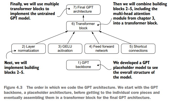
我们将按照上图的流程一步步的构建GPT architecture。

首先用字典存一下gpt-2的一些参数设置：

python 复制代码

GPT_CONFIG_124M = {
    "vocab_size": 50257, # Vocabulary size
    "context_length": 1024, # Context length
    "emb_dim": 768, # Embedding dimension
    "n_heads": 12, # Number of attention heads
    "n_layers": 12, # Number of layers
    "drop_rate": 0.1, # Dropout rate
    "qkv_bias": False # Query-Key-Value bias
}

然后搭一下backbone：

python 复制代码

import torch
import torch.nn as nn

class DummyTransformerBlock(nn.Module):
    def __init__(self, cfg):
        super().__init__()
    def forward(self, x):
        return x
class DummyLayerNorm(nn.Module):
    def __init__(self, normalized_shape, eps=1e-5):
        super().__init__()
    def forward(self, x):
        return x

class DummyGPTModel(nn.Module):
    def __init__(self, cfg):
        super().__init__()
        self.tok_emb = nn.Embedding(cfg["vocab_size"], cfg["emb_dim"])
        self.pos_emb = nn.Embedding(cfg["context_length"], cfg["emb_dim"])
        self.drop_emb = nn.Dropout(cfg["drop_rate"])
        self.trf_blocks = nn.Sequential(
            *[DummyTransformerBlock(cfg)
                for _ in range(cfg["n_layers"])]
        )
        self.final_norm = DummyLayerNorm(cfg["emb_dim"])
        self.out_head = nn.Linear(
            cfg["emb_dim"], cfg["vocab_size"], bias = False
        )
    
    def forward(self, in_idx):
        batch_size, seq_len = in_idx.shape
        tok_embeds = self.tok_emb(in_idx)
        pos_embeds = self.pos_emb(
            torch.arange(seq_len, device = in_idx.device)
        ) # [0, 1, .., seq_len-1]
        x = tok_embeds + pos_embeds
        x = self.drop_emb(x)
        x = self.trf_blocks(x)
        x = self.final_norm(x)
        logits = self.out_head(x)
        return logits

DummyTransformerBlock 和 DummyLayerNorm只是暂时占位，后面会补充实现
DummyGPTModel 的架构还是比较简单的

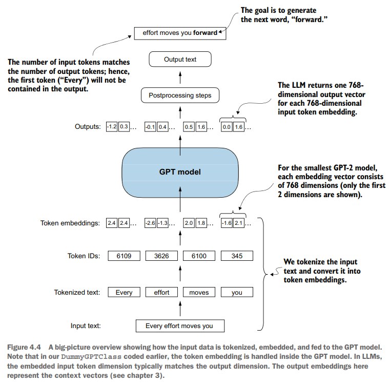
GPT-model的数据流如下：

为了实践，下面利用ch-02的tokenizer造一些样例：

python 复制代码

import tiktoken

tokenizer = tiktoken.get_encoding("gpt2")
batch = []
txt1 = "Every effort moves you"
txt2 = "Every day holds a"

batch.append(torch.tensor(tokenizer.encode(txt1)))
batch.append(torch.tensor(tokenizer.encode(txt2)))
batch = torch.stack(batch, dim=0)
batch

复制代码

tensor([[6109, 3626, 6100,  345],
        [6109, 1110, 6622,  257]])

python 复制代码

torch.manual_seed(123)
model = DummyGPTModel(GPT_CONFIG_124M)
logits = model(batch)
print("Output shape:", logits.shape)
print(logits)

复制代码

Output shape: torch.Size([2, 4, 50257])
tensor([[[-1.2034,  0.3201, -0.7130,  ..., -1.5548, -0.2390, -0.4667],
         [-0.1192,  0.4539, -0.4432,  ...,  0.2392,  1.3469,  1.2430],
         [ 0.5307,  1.6720, -0.4695,  ...,  1.1966,  0.0111,  0.5835],
         [ 0.0139,  1.6755, -0.3388,  ...,  1.1586, -0.0435, -1.0400]],

        [[-1.0908,  0.1798, -0.9484,  ..., -1.6047,  0.2439, -0.4530],
         [-0.7860,  0.5581, -0.0610,  ...,  0.4835, -0.0077,  1.6621],
         [ 0.3567,  1.2698, -0.6398,  ..., -0.0162, -0.1296,  0.3717],
         [-0.2407, -0.7349, -0.5102,  ...,  2.0057, -0.3694,  0.1814]]],
       grad_fn=<UnsafeViewBackward0>)

1.2 layer normalization

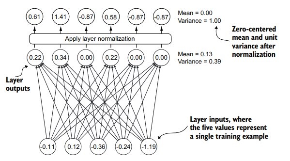
为了降低梯度衰退或者爆炸，我们要实现一个 layer normalization来提高模型的稳定性以及训练的效率。

在GPT-2以及现代transformer 架构中，层归一化往往在多头注意力之前或者之后进行。

先来创建几个样例：

python 复制代码

torch.manual_seed(123)
batch_example = torch.randn(2, 5)
layer = nn.Sequential(nn.Linear(5, 6), nn.ReLU())
out = layer(batch_example)
out

复制代码

tensor([[0.2260, 0.3470, 0.0000, 0.2216, 0.0000, 0.0000],
        [0.2133, 0.2394, 0.0000, 0.5198, 0.3297, 0.0000]],
       grad_fn=<ReluBackward0>)

python 复制代码

mean = out.mean(dim=-1, keepdim=True)
var = out.var(dim=-1, keepdim=True)
print("Mean:\n", mean)
print("Variance:\n", var)

复制代码

Mean:
 tensor([[0.1324],
        [0.2170]], grad_fn=<MeanBackward1>)
Variance:
 tensor([[0.0231],
        [0.0398]], grad_fn=<VarBackward0>)

keepdim 保证返回的结果的维度数目不变，比如上面的mean如果keepdim=False 返回的就会是 $0.1324, 0.2170$

然后我们可以对其进行层归一化：

python 复制代码

out_norm = (out - mean) / torch.sqrt(var)
mean = out_norm.mean(dim=-1, keepdim=True)
var = out_norm.var(dim=-1, keepdim=True)
print("Normalized layer outputs:\n", out_norm)
print("Mean:\n", mean)
print("Variance:\n", var)

复制代码

Normalized layer outputs:
 tensor([[ 0.6159,  1.4126, -0.8719,  0.5872, -0.8719, -0.8719],
        [-0.0189,  0.1121, -1.0876,  1.5173,  0.5647, -1.0876]],
       grad_fn=<DivBackward0>)
Mean:
 tensor([[9.9341e-09],
        [0.0000e+00]], grad_fn=<MeanBackward1>)
Variance:
 tensor([[1.0000],
        [1.0000]], grad_fn=<VarBackward0>)

--5.9605e-08 是科学计数法表示，其实已经很接近0了，我们可以设置 sci_mode = False：

python 复制代码

torch.set_printoptions(sci_mode=False)
print("Mean:\n", mean)
print("Variance:\n", var)

复制代码

Mean:
 tensor([[0.0000],
        [0.0000]], grad_fn=<MeanBackward1>)
Variance:
 tensor([[1.0000],
        [1.0000]], grad_fn=<VarBackward0>)

最后只需要把这些操作包装成类即可：

python 复制代码

class LayerNorm(nn.Module):
    def __init__(self, emb_dim):
        super().__init__()
        self.eps = 1E-5
        self.scale = nn.Parameter(torch.ones(emb_dim))
        self.shift = nn.Parameter(torch.zeros(emb_dim))
    
    def forward(self, x):
        mean = x.mean(dim=-1, keepdim=True)
        var = x.var(dim=-1, keepdim=True, unbiased=False)
        norm_x = (x - mean) / torch.sqrt(var + self.eps)
        return self.scale * norm_x + self.shift

Q：代码里的eps、scale、shift是干嘛的

A：

eps为了防止除0异常

scale和shift则是让模型在训练的时候决定是否通过缩放和偏置来更好的适配数据。

测试一下：

python 复制代码

ln = LayerNorm(emb_dim=5)
out_ln = ln(batch_example)
mean = out_ln.mean(dim=-1, keepdim=True)
var = out_ln.var(dim=-1, unbiased=False, keepdim=True)
print("Mean:\n", mean)
print("Variance:\n", var)

复制代码

Mean:
 tensor([[-0.0000],
        [ 0.0000]], grad_fn=<MeanBackward1>)
Variance:
 tensor([[1.0000],
        [1.0000]], grad_fn=<VarBackward0>)

Q：为什么LayerNorm 中加了 unbiased参数？

A：Biased variance 在计算 variance时用分母不是 n 而是 n - 1，这和概率统计课程中的无偏性有关。

但是对于LLM这样的大数据训练模型，n 和 n - 1几乎没差别，那么根据大数定律，我们用n即可。

作者增加这个参数是因为GPT-2的参数基于Tensorflow，保留这个参数是为了后面章节加载预训练权重时保持一致。
Q：Layer normalization vs. batch normalization

A：

层归一化：沿着特征维度做归一化

批量归一化：沿着 batch 的维度做归一化

相比于 batchnorm，layernorm：

不依赖 batch size，小 batch 也稳定

训练和推理行为一致

BatchNorm 在训练和推理时行为不同。训练时：用当前 batch 的 mean / var；推理时：用训练过程中累计的 running_mean / running_var

更适合序列模型和 NLP

NLP 任务中的 batch 经常有：不同句子长度；padding；动态 batch；自回归生成；batch size 受显存限制；token 分布差异很大。

适合自回归生成

GPT 这种模型推理时是一个 token 一个 token 地生成。用BatchNorm就得考虑：当前 batch 的统计量是什么？序列长度变了怎么办？训练时和生成时统计是否一致？

不受 batch 内样本相互影响

分布式训练更方便。BatchNorm 在多 GPU 训练时，如果每张卡上的 batch size 很小，那么每张卡算出来的 BatchNorm 统计量会不稳定。可以用 SyncBatchNorm 在多卡之间同步统计，但这会增加通信开销。LayerNorm 不需要跨样本统计，也不需要跨 GPU 同步，因此分布式训练更简单。

更适合 Transformer 的残差结构。LayerNorm 对每个 token 的 hidden vector 做归一化，可以稳定每层的激活尺度，使深层 Transformer 更容易训练。

1.3 feed forward network with GELU activations

作者首先介绍了 GELU，初学者一般更熟悉 ReLU，GELU和ReLU的作用相同，只不过式子更复杂，曲线更加的平滑：

G E L U ( x ) ≈ 0.5 ⋅ x ⋅ ( 1 + t a n h $2 π \cdot ( x + 0.044715 \cdot x 3 )$ ) GELU(x) \approx 0.5 \cdot x \cdot \left ( 1 + tanh\lbrack \sqrt{\frac{2}{\pi }}\cdot (x + 0.044715 \cdot x^3) \rbrack \right ) GELU(x)≈0.5⋅x⋅(1+tanh $π2 \cdot(x+0.044715\cdotx3)$ )

写一个GELU类：

python 复制代码

class GELU(nn.Module):
    def __init__(self):
        super().__init__()
    
    def forward(self, x):
        return 0.5 * x * (1 + torch.tanh(torch.sqrt(torch.tensor(2.0 / torch.pi)) * (x + 0.044715 * torch.pow(x, 3))))

画图对比：

python 复制代码

import matplotlib.pyplot as plt
gelu, relu = GELU(), nn.ReLU()

x = torch.linspace(-3, 3, 100)
y_gelu, y_relu = gelu(x), relu(x)
plt.figure(figsize=(8, 3))
for i, (y, label) in enumerate(zip([y_gelu, y_relu], ["GELU", "ReLU"]), 1):
    plt.subplot(1, 2, i)
    plt.plot(x, y)
    plt.title(f"{label} activation function")
    plt.xlabel("x")
    plt.ylabel(f"{label}(x)")
    plt.grid(True)
plt.tight_layout()
plt.show()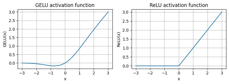

GELU的平滑性可以使得model在训练过程中进行更好的optimize。

而且，ReLU对于负数映射到0，而GELU会给出一个非0值。

下面基于GELU来搓一个FeedForward：

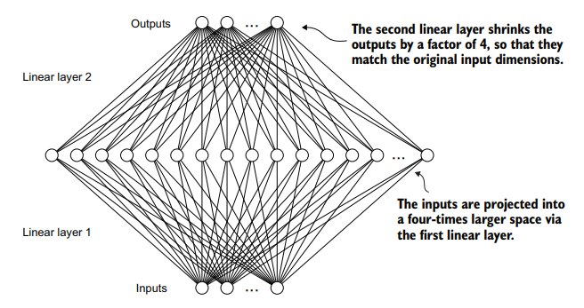
FeedForward就是一个两层的小神经网络

先将输入向量扩展到高维语义空间，然后再提取信息，返回输入维度的向量空间。

python 复制代码

class FeedForward(nn.Module):
    def __init__(self, cfg):
        super().__init__()
        self.layers = nn.Sequential(
            nn.Linear(cfg["emb_dim"], 4 * cfg["emb_dim"]),
            GELU(),
            nn.Linear(4 * cfg["emb_dim"], cfg["emb_dim"]),
        )
    
    def forward(self, x):
        return self.layers(x)

python 复制代码

ffn = FeedForward(GPT_CONFIG_124M)
x = torch.rand(2, 3, 768)
out = ffn(x)
out.shape

复制代码

torch.Size([2, 3, 768])

1.4 Adding shortcut connections

作者花了一些篇幅来讲残差连接。

最早是在ResNet中提出，在深层的神经网络中可以有效地应对梯度消失。

然后就是写了一个简单的5层神经网络，分别对比了加入shortcut前和加入shortcut后的梯度：

python 复制代码

class ExampleDeepNeuralNetwork(nn.Module):
    def __init__(self, layer_sizes, use_shortcut):
        super().__init__()
        self.use_shortcut = use_shortcut
        self.layers = nn.ModuleList([
            nn.Sequential(nn.Linear(layer_sizes[0], layer_sizes[1]), GELU()),
            nn.Sequential(nn.Linear(layer_sizes[1], layer_sizes[2]), GELU()),
            nn.Sequential(nn.Linear(layer_sizes[2], layer_sizes[3]), GELU()),
            nn.Sequential(nn.Linear(layer_sizes[3], layer_sizes[4]), GELU()),
            nn.Sequential(nn.Linear(layer_sizes[4], layer_sizes[5]), GELU())
        ])

    def forward(self, x):
        for layer in self.layers:
            # Compute the output of the current layer
            layer_output = layer(x)
            # Check if shortcut can be applied
            if self.use_shortcut and x.shape == layer_output.shape:
                x = x + layer_output
            else:
                x = layer_output
        return x


def print_gradients(model, x):
    # Forward pass
    output = model(x)
    target = torch.tensor([[0.]])

    # Calculate loss based on how close the target
    # and output are
    loss = nn.MSELoss()
    loss = loss(output, target)
    
    # Backward pass to calculate the gradients
    loss.backward()

    for name, param in model.named_parameters():
        if 'weight' in name:
            # Print the mean absolute gradient of the weights
            print(f"{name} has gradient mean of {param.grad.abs().mean().item()}")

python 复制代码

layer_sizes = [3, 3, 3, 3, 3, 1]
sample_input = torch.tensor([[1., 0., -1.]])
torch.manual_seed(123)
model_without_shortcut = ExampleDeepNeuralNetwork(
 layer_sizes, use_shortcut=False
)
print_gradients(model_without_shortcut, sample_input)

复制代码

layers.0.0.weight has gradient mean of 0.00020173587836325169
layers.1.0.weight has gradient mean of 0.0001201116101583466
layers.2.0.weight has gradient mean of 0.0007152041653171182
layers.3.0.weight has gradient mean of 0.001398873864673078
layers.4.0.weight has gradient mean of 0.005049646366387606

python 复制代码

torch.manual_seed(123)
model_with_shortcut = ExampleDeepNeuralNetwork(
    layer_sizes, use_shortcut=True
)
print_gradients(model_with_shortcut, sample_input)

复制代码

layers.0.0.weight has gradient mean of 0.2216978669166565
layers.1.0.weight has gradient mean of 0.20694100856781006
layers.2.0.weight has gradient mean of 0.3289698660373688
layers.3.0.weight has gradient mean of 0.2665731906890869
layers.4.0.weight has gradient mean of 1.3258538246154785

可见，加入shortcut后，梯度的值明显有所上升。

1.5 transformer block

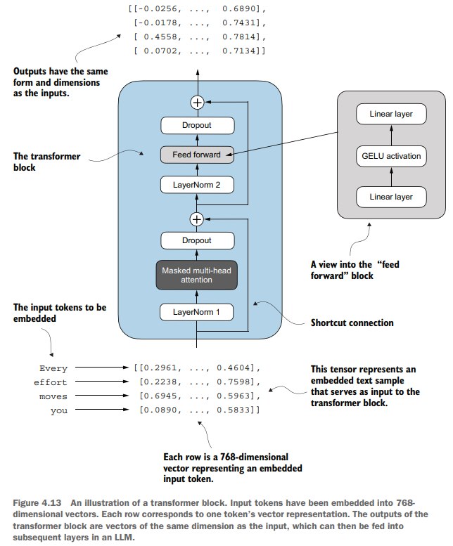
然后终于可以开始编写 transformer block，主要就是整合了一下前面写的块。

在124M的GPT-2 model中，transformer block 重复了12次，结合了多头注意力机制、layer norm、dropout、feed forward layer。

这使得模型能够更好地理解和处理输入，同时增强了模型总体的复杂数据模式处理能力。

GPT-2 所采用的transformer 架构：

实现一下transformer block：

python 复制代码

from previous_chapters import MultiHeadAttention

class TransformerBlock(nn.Module):
    def __init__(self, cfg):
        super().__init__()
        self.att = MultiHeadAttention(
            d_in=cfg["emb_dim"],
            d_out=cfg["emb_dim"],
            context_length=cfg["context_length"],
            num_heads=cfg["n_heads"],
            dropout=cfg["drop_rate"],
            qkv_bias=cfg["qkv_bias"])
        self.ff = FeedForward(cfg)
        self.norm1 = LayerNorm(cfg["emb_dim"])
        self.norm2 = LayerNorm(cfg["emb_dim"])
        self.drop_shortcut = nn.Dropout(cfg["drop_rate"])
    
    def forward(self, x):
        # Shortcut connection for attention block
        shortcut = x
        x = self.norm1(x)
        x = self.att(x)
        x = self.drop_shortcut(x)
        x += shortcut

        # shortcut connection for feed forward block
        shortcut = x
        x = self.norm2(x)
        x = self.ff(x)
        x = self.drop_shortcut(x)
        x += shortcut
        return x

python 复制代码

torch.manual_seed(123)
x = torch.rand(2, 4, 768)
block = TransformerBlock(GPT_CONFIG_124M)
output = block(x)

print("Input shape:", x.shape)
print("Output shape:", output.shape)

复制代码

Input shape: torch.Size([2, 4, 768])
Output shape: torch.Size([2, 4, 768])

transformer block 保持了输入向量的维度，即不会改变输入数据的shape。

这并不是偶然，反而是一个重要的设计。这一设计使其能够有效应用于广泛的序列到序列任务，其中每个输出向量与一个输入向量直接对应，维持着一对一的关系。然而，输出实际上是一个上下文向量，它封装了来自整个输入序列的信息。

这意味着，当序列通过Transformer模块时，其维度虽保持不变，但每个输出向量的内容被重新编码，以整合来自整个输入序列的上下文信息。

1.6 Coding the GPT model

本章开始的时候，编写了一个GPT架构的总览：DummyGPTModel。不过当时的transformer block和layernorm都是空壳。

现在需要用的模块都已实现，可以真正地实现GPT model了。

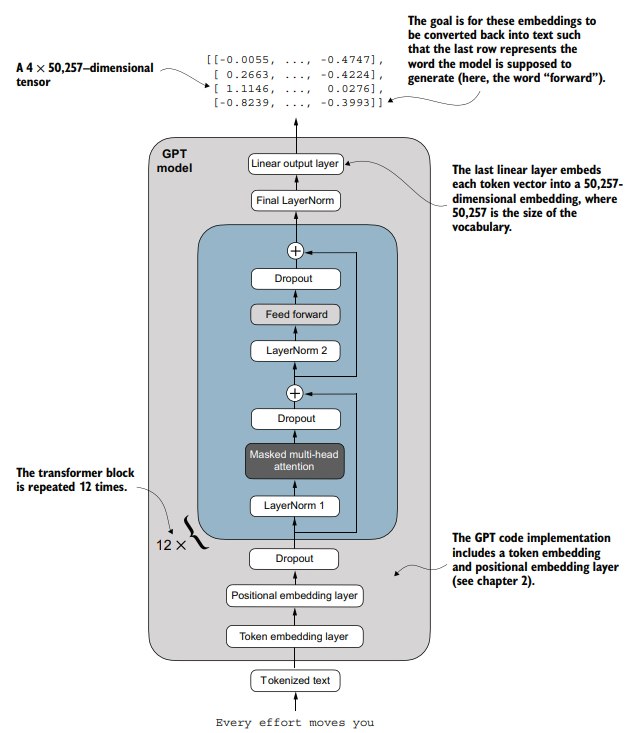
现在可以把gpt model的架构更为详细地进行展示：

然后组装：

python 复制代码

class GPTModel(nn.Module):
    def __init__(self, cfg):
        super().__init__()
        self.tok_emb = nn.Embedding(cfg["vocab_size"], cfg["emb_dim"])
        self.pos_emb = nn.Embedding(cfg["context_length"], cfg["emb_dim"])
        self.drop_emb = nn.Dropout(cfg["drop_rate"])

        self.trf_blocks = nn.Sequential(
            *[TransformerBlock(cfg) for _ in range(cfg["n_layers"])]
        )

        self.final_norm = LayerNorm(cfg["emb_dim"])
        self.out_head = nn.Linear(
            cfg["emb_dim"], cfg["vocab_size"], bias=False
        )

    def forward(self, in_idx):
        batch_size, seq_len = in_idx.shape
        tok_embeds = self.tok_emb(in_idx)
        
        # train the model on CPU or GPU depends on which device the input data sits on
        pos_embeds = self.pos_emb(
            torch.arange(seq_len, device=in_idx.device)
        )

        x = tok_embeds + pos_embeds
        x = self.drop_emb(x)
        x = self.trf_blocks(x)
        x = self.final_norm(x)
        # we get logits for each word
        logits = self.out_head(x)
        return logits

然后用124M gpt-model配置来初始化，并对最开始创建那个batch进行测试：

python 复制代码

torch.manual_seed(123)
model = GPTModel(GPT_CONFIG_124M)

out = model(batch)
print("Input batch:\n", batch)
print("\nOutput shape:", out.shape)
print(out)

复制代码

Input batch:
 tensor([[6109, 3626, 6100,  345],
        [6109, 1110, 6622,  257]])

Output shape: torch.Size([2, 4, 50257])
tensor([[[ 0.3613,  0.4222, -0.0711,  ...,  0.3483,  0.4661, -0.2838],
         [-0.1792, -0.5660, -0.9485,  ...,  0.0477,  0.5181, -0.3168],
         [ 0.7120,  0.0332,  0.1085,  ...,  0.1018, -0.4327, -0.2553],
         [-1.0076,  0.3418, -0.1190,  ...,  0.7195,  0.4023,  0.0532]],

        [[-0.2564,  0.0900,  0.0335,  ...,  0.2659,  0.4454, -0.6806],
         [ 0.1230,  0.3653, -0.2074,  ...,  0.7705,  0.2710,  0.2246],
         [ 1.0558,  1.0318, -0.2800,  ...,  0.6936,  0.3205, -0.3178],
         [-0.1565,  0.3926,  0.3288,  ...,  1.2630, -0.1858,  0.0388]]],
       grad_fn=<UnsafeViewBackward0>)

模型最终为每个输入token计算了一个词表的logits，用于后续的分类输出。

我们可以看一下我们手写的GPTModel的参数量：

python 复制代码

total_params = sum(p.numel() for p in model.parameters())
print(f"Total number of parameters: {total_params:,}")

复制代码

Total number of parameters: 163,009,536

发现大概在163M左右，为什么呢？

原始的GPT-2 架构在最后的输出层复用了token embedding矩阵，我们不妨分别打印一下Token embedding layer和Output layer 的shape：

python 复制代码

print("Token embedding layer shape:", model.tok_emb.weight.shape)
print("Output layer shape:", model.out_head.weight.shape)

复制代码

Token embedding layer shape: torch.Size([50257, 768])
Output layer shape: torch.Size([50257, 768])

那我们不妨计算一下除了输出头的参数量：

python 复制代码

total_params_gpt2 =  total_params - sum(p.numel() for p in model.out_head.parameters())
print(f"Number of trainable parameters considering weight tying: {total_params_gpt2:,}")

复制代码

Number of trainable parameters considering weight tying: 124,412,160

顺带计算一下需要多大存储：

python 复制代码

# Calculate the total size in bytes (assuming float32, 4 bytes per parameter)
total_size_bytes = total_params * 4

# Convert to megabytes
total_size_mb = total_size_bytes / (1024 * 1024)

print(f"Total size of the model: {total_size_mb:.2f} MB")

复制代码

Total size of the model: 621.83 MB

4.7 Generating text

现在我们的GPTModel 对于一个输入可以生成对应的词表的logits作为输出。

所以我们真的要去生成文本时，还需要将logits通过softmax转化为概率，然后进一步地输出文本。

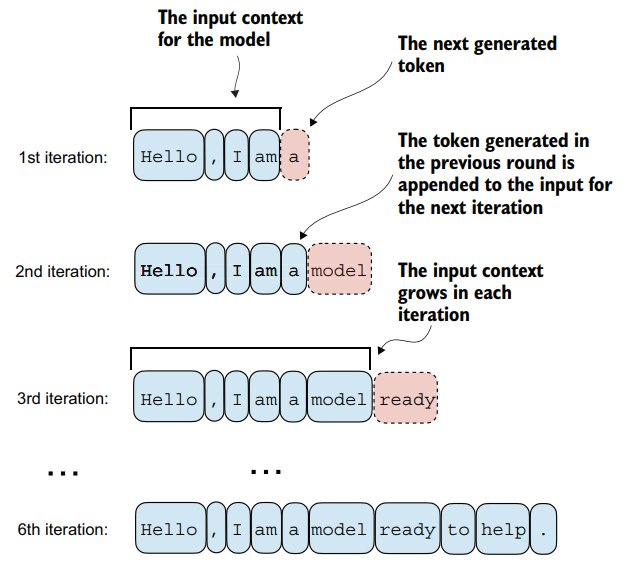
写一个接受输入，并输出预测token id的函数：

python 复制代码

def generate_text_simple(model, idx, max_new_tokens, contex_size):
    for _ in range(max_new_tokens):
        idx_cond = idx[:, -contex_size:]
        with torch.no_grad():
            logits = model(idx_cond)
        
        logits = logits[:, -1, :]
        probas = torch.softmax(logits, dim=-1)
        idx_next = torch.argmax(probas, dim=-1, keepdim=True)
        idx = torch.cat((idx, idx_next), dim=1)
    return idx

写个例子测试下：

python 复制代码

start_context = "Hello, I am"
encoded = tokenizer.encode(start_context)
print("encoded:", encoded)
encoded_tensor = torch.tensor(encoded).unsqueeze(0)
print("encoded_tensor.shape:", encoded_tensor.shape)

复制代码

encoded: [15496, 11, 314, 716]
encoded_tensor.shape: torch.Size([1, 4])

模型预测下：

python 复制代码

model.eval()
out = generate_text_simple(
    model=model,
    idx=encoded_tensor,
    max_new_tokens=6,
    contex_size=GPT_CONFIG_124M["context_length"]
)
print("Output:", out)
print("Output length:", len(out[0]))

复制代码

Output: tensor([[15496,    11,   314,   716, 27018, 24086, 47843, 30961, 42348,  7267]])
Output length: 10

转文本：

python 复制代码

decoded_text = tokenizer.decode(out.squeeze(0).tolist())
print(decoded_text)

复制代码

Hello, I am Featureiman Byeswickattribute argue

这个输出并不是我们预期的，这是因为我们没有做预训练，这将在下一章进行。