step1 配置对应的库
python
import torch
from torchvision import transforms, datasets
from torch.utils.data import DataLoader
import matplotlib.pyplot as plt
#隐藏警告
import warnings
warnings.filterwarnings("ignore")               #忽略警告信息

plt.rcParams['font.sans-serif']    = ['SimHei'] # 用来正常显示中文标签
plt.rcParams['axes.unicode_minus'] = False      # 用来正常显示负号
plt.rcParams['figure.dpi']         = 100        #分辨率


device = torch.device("cuda" if torch.cuda.is_available() else "cpu")
device
step2 读取(下载)MNIST数据集
python
transform = transforms.Compose([transforms.ToTensor(), transforms.Normalize((0.1307,), (0.3081,))])

train_dataset = datasets.MNIST(root='../datasets/mnist', train=True, download=True, transform=transform)  # download=True:如果没有下载数据集
test_dataset = datasets.MNIST(root='../datasets/mnist', train=False, download=True, transform=transform)  # train=True训练集,=False测试集
创建数据加载器
python
batch_size = 32

train_loader = DataLoader(train_dataset, batch_size=batch_size, shuffle=True)
test_loader = DataLoader(test_dataset, batch_size=batch_size, shuffle=False)
step3 展示MNIST数据集
python
import matplotlib.pyplot as plt

# 只加载部分数据到内存
fig = plt.figure(figsize=(12, 8))
for i in range(12):
    # 每次只访问单个样本,不提前加载全部
    img, label = train_dataset[i]
    plt.subplot(3, 4, i+1)
    plt.imshow(img.squeeze().numpy(), cmap='gray', interpolation='none')
    plt.title(f"Label: {label}")
    plt.xticks([])
    plt.yticks([])
plt.tight_layout()
plt.show()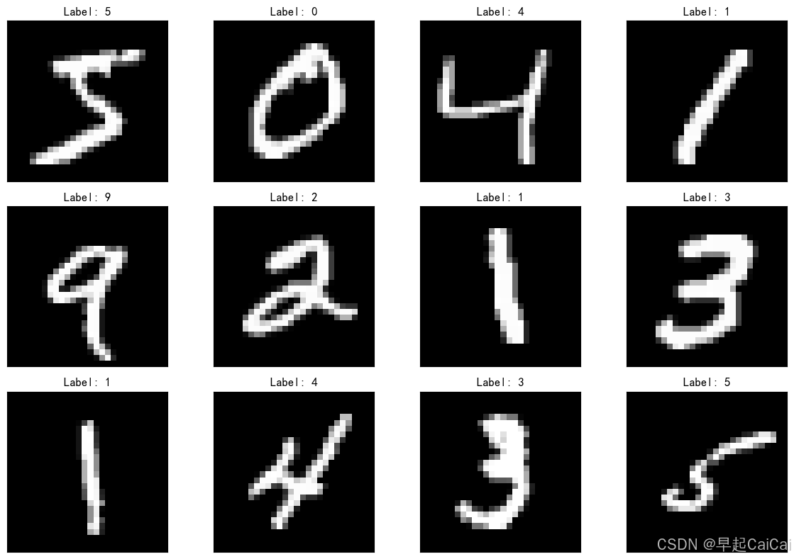
step4 构建简单的CNN网络
python
class Net(torch.nn.Module):
    def __init__(self):
        # (batch,1,28,28)
        super(Net, self).__init__()
        self.conv1 = torch.nn.Sequential(
            torch.nn.Conv2d(1, 32, kernel_size=3), #(batch,32,26,26) 输入通道数1输出通道数32 32为小型任务的经验性选择,一般每层增加一倍欠拟合就加过拟合减
            torch.nn.BatchNorm2d(32),              # 对卷积层的输出进行批量归一化,使得每个特征图的分布更加稳定,从而加速训练并提高模型性能。
            torch.nn.ReLU(),
            torch.nn.MaxPool2d(kernel_size=2), #(batch,32,13,13)
        )
        self.conv2 = torch.nn.Sequential(
            torch.nn.Conv2d(32, 64, kernel_size=3), #(batch,64,11,11)
            torch.nn.BatchNorm2d(64),
            torch.nn.ReLU(),
            torch.nn.MaxPool2d(kernel_size=2), #(batch,64,5,5)
        )
        self.fc = torch.nn.Sequential(
            torch.nn.Linear(1600, 50), # 1600 == 64*5*5
            torch.nn.ReLU(),  # 添加ReLU激活函数 增加模型的非线性能力
            torch.nn.Dropout(0.5), # 有效防止过拟合-丢弃率0.5          BN层和dropout层一起用效果不好( 深层可能不好BN在后Dropout在前也不好
            torch.nn.Linear(50, 10)
        )

    def forward(self, x):
        batch_size = x.size(0)
        x = self.conv1(x)  # 一层卷积层,一层池化层,一层激活层
        x = self.conv2(x)  # 再来一次
        x = x.view(batch_size, -1)  # flatten 变成全连接网络需要的输入
        x = self.fc(x)
        return x  # 最后输出的是维度为10的,也就是(对应数学符号的0~9)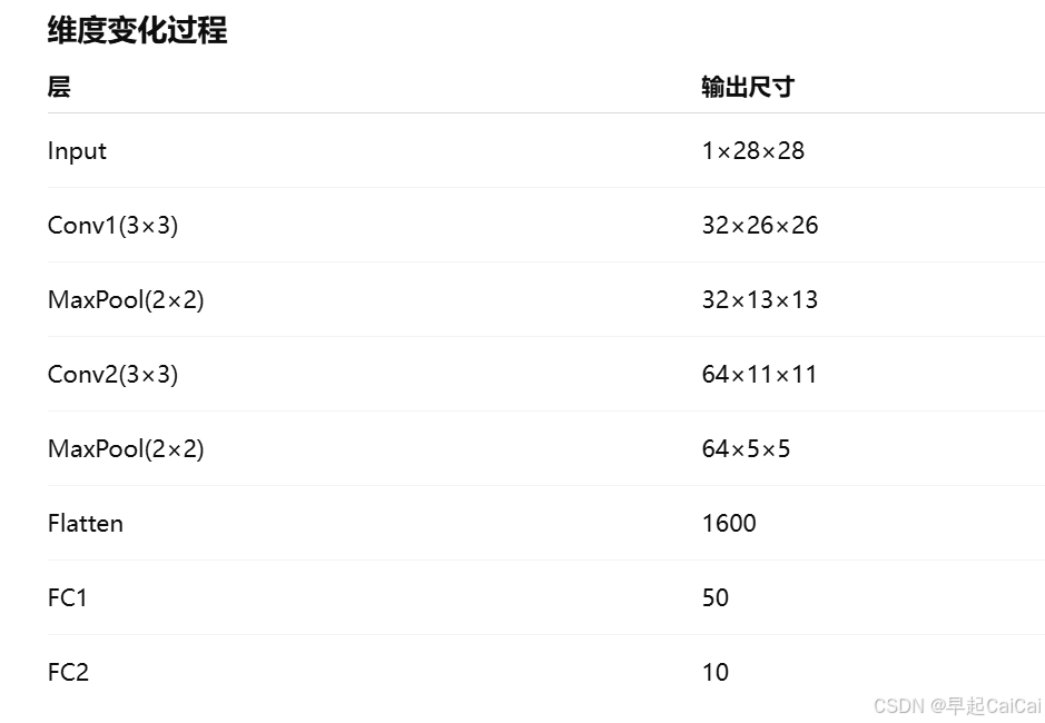
python
model = Net().to(device)

# 查看模型结构
# 打印模型参数总数和可训练参数总数
def count_parameters(model):
    total_params = sum(p.numel() for p in model.parameters())  # 所有参数数量
    trainable_params = sum(p.numel() for p in model.parameters() if p.requires_grad)  # 需要训练的参数数量
    print(f"模型总参数数量: {total_params:,}")
    print(f"模型可训练参数数量: {trainable_params:,}")

print(model)
count_parameters(model)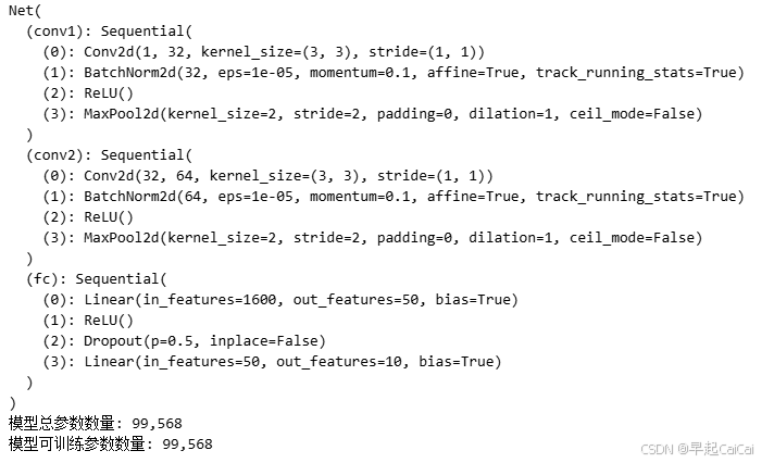
step5 训练模型
python
loss_fn    = torch.nn.CrossEntropyLoss() # 交叉熵损失函数,常用在多分类任务中
learn_rate = 0.01 # 学习率
optimizer  = torch.optim.SGD(model.parameters(), lr=learn_rate, momentum = 0.9)
python
# 训练循环
def train(dataloader, model, loss_fn, optimizer):
    size = len(dataloader.dataset)  # 训练集的大小,一共60000张图片
    num_batches = len(dataloader)   # 批次数目,1875(60000/32)

    train_loss, train_acc = 0, 0  # 初始化训练损失和正确率

    for X, y in dataloader:  # 获取图片及其标签
        X, y = X.to(device), y.to(device)

        # 计算预测误差
        pred = model(X)          # 网络输出
        loss = loss_fn(pred, y)  # 计算网络输出和真实值之间的差距,targets为真实值,计算二者差值即为损失

        # 反向传播
        optimizer.zero_grad()  # grad属性归零
        loss.backward()        # 反向传播
        optimizer.step()       # 每一步自动更新

        # 记录acc与loss
        train_acc  += (pred.argmax(1) == y).type(torch.float).sum().item()
        train_loss += loss.item()

    train_acc  /= size
    train_loss /= num_batches

    return train_acc, train_loss
python
def test(dataloader, model, loss_fn):
    size        = len(dataloader.dataset)  # 测试集的大小,一共10000张图片
    num_batches = len(dataloader)          # 批次数目,313(10000/32=312.5,向上取整)
    test_loss, test_acc = 0, 0

    # 当不进行训练时,停止梯度更新,节省计算内存消耗
    with torch.no_grad():
        for imgs, target in dataloader:
            imgs, target = imgs.to(device), target.to(device)

            # 计算loss
            target_pred = model(imgs)
            loss        = loss_fn(target_pred, target)

            test_loss += loss.item()
            test_acc  += (target_pred.argmax(1) == target).type(torch.float).sum().item()

    test_acc  /= size
    test_loss /= num_batches

    return test_acc, test_loss
step 6 开始训练
模型会对整个训练集学习100遍
python
epochs     = 100
train_loss = []
train_acc  = []
test_loss  = []
test_acc   = []

for epoch in range(epochs):
    model.train()
    epoch_train_acc, epoch_train_loss = train(train_loader, model, loss_fn, optimizer)

    model.eval()
    epoch_test_acc, epoch_test_loss = test(test_loader, model, loss_fn)

    train_acc.append(epoch_train_acc)
    train_loss.append(epoch_train_loss)
    test_acc.append(epoch_test_acc)
    test_loss.append(epoch_test_loss)

    template = ('Epoch:{:2d}, Train_acc:{:.1f}%, Train_loss:{:.3f}, Test_acc:{:.1f}%,Test_loss:{:.3f}')
    print(template.format(epoch+1, epoch_train_acc*100, epoch_train_loss, epoch_test_acc*100, epoch_test_loss))
step7 结果可视化
python
epochs_range = range(epochs)

plt.figure(figsize=(12, 3))
plt.subplot(1, 2, 1)

plt.plot(epochs_range, train_acc, label='Training Accuracy')
plt.plot(epochs_range, test_acc, label='Test Accuracy')
plt.legend(loc='lower right')
plt.title('Training and Validation Accuracy')

plt.subplot(1, 2, 2)
plt.plot(epochs_range, train_loss, label='Training Loss')
plt.plot(epochs_range, test_loss, label='Test Loss')
plt.legend(loc='upper right')
plt.title('Training and Validation Loss')
plt.show()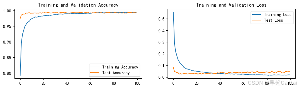
大概在40次最优
step8 保存模型和加载模型
python
# 指定保存路径
save_dir = './models/1_Handwritten_Digit_Recognition'

# 确保目录存在,如果不存在则创建
import os
if not os.path.exists(save_dir):
    os.makedirs(save_dir)

# 保存模型
torch.save(model.state_dict(), os.path.join(save_dir, 'model_weights.pth'))

# # 加载模型参数
# model.load(torch.load(os.path.join(save_dir, 'model_weights.pth')))
数字识别
利用训练好的模型进行数字识别
python
import torch
from PIL import Image
import torchvision.transforms as transforms

device = torch.device("cuda" if torch.cuda.is_available() else "cpu")
device
python
class Net(torch.nn.Module):
    def __init__(self):
        # (batch,1,28,28)
        super(Net, self).__init__()
        self.conv1 = torch.nn.Sequential(
            torch.nn.Conv2d(1, 32, kernel_size=3), #(batch,32,26,26) 输入通道数1输出通道数32 32为小型任务的经验性选择,一般每层增加一倍欠拟合就加过拟合减
            torch.nn.BatchNorm2d(32),              # 对卷积层的输出进行批量归一化,使得每个特征图的分布更加稳定,从而加速训练并提高模型性能。
            torch.nn.ReLU(),
            torch.nn.MaxPool2d(kernel_size=2), #(batch,32,13,13)
        )
        self.conv2 = torch.nn.Sequential(
            torch.nn.Conv2d(32, 64, kernel_size=3), #(batch,64,11,11)
            torch.nn.BatchNorm2d(64),
            torch.nn.ReLU(),
            torch.nn.MaxPool2d(kernel_size=2), #(batch,64,5,5)
        )
        self.fc = torch.nn.Sequential(
            torch.nn.Linear(1600, 50), # 1600 == 64*5*5
            torch.nn.ReLU(),           # 添加ReLU激活函数 增加模型的非线性能力
            torch.nn.Dropout(0.5),     # 有效防止过拟合-丢弃率0.5          BN层和dropout层一起用效果不好( 深层可能不好BN在后Dropout在前也不好
            torch.nn.Linear(50, 10)
        )

    def forward(self, x):
        batch_size = x.size(0)
        x = self.conv1(x)  # 一层卷积层,一层池化层,一层激活层
        x = self.conv2(x)  # 再来一次
        x = x.view(batch_size, -1)  # flatten 变成全连接网络需要的输入
        x = self.fc(x)
        return x  # 最后输出的是维度为10的,也就是(对应数学符号的0~9)
python
model = Net().to(device)

model_path = './models/1_Handwritten_Digit_Recognition/model_weights.pth'

# 加载模型参数
model.load_state_dict(torch.load(model_path, map_location=device))

# 将模型设置为评估模式
model.eval()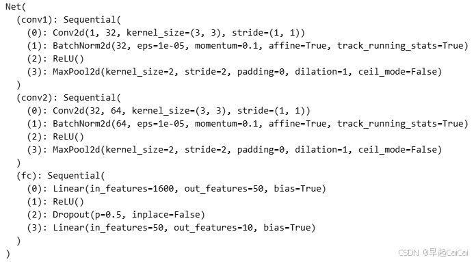
python
# 预测函数
def predict_image(image_path, model):
    image = Image.open(image_path)
    # 图像预处理
    transform = transforms.Compose([
        transforms.Grayscale(num_output_channels=1),  # 转换为灰度
        transforms.Resize((28, 28)),                 # 调整到 28x28
        transforms.ToTensor(),                       # 转换为张量
        transforms.Normalize((0.5,), (0.5,))         # 归一化到 [-1, 1]
    ])
    image = transform(image)
    image = image.to(device)
    image = image.unsqueeze(0)

    with torch.no_grad():
        output = model(image)
        _, predicted = torch.max(output.data, 1)
    return predicted.item()
python
#展示图片
import matplotlib.pyplot as plt
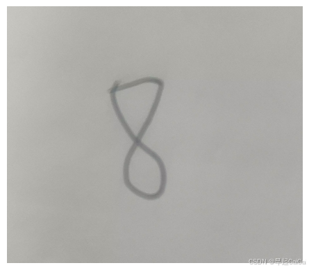
img = Image.open('./data/8.png')
# 显示图像
plt.imshow(img)
plt.axis('off') # 可选,关闭坐标轴
# plt.show()
# 使用模型进行预测
predicted_digit = predict_image('./data/8.png', model)
print(f"Predicted digit: {predicted_digit}")模型准备度不够,识别为7(貌似对8的识别误差较大)
能识别为2

多个数字识别
python
import cv2
import numpy as np
import matplotlib.pyplot as plt
step1 图形加载
python
image = cv2.imread('./data/5678.png', cv2.IMREAD_GRAYSCALE) # cv2.IMREAD_GRAYSCALE表示加载为灰度图像

# 二值化
"""
黑色(0) 白色(255)
127是阈值
255是大于阈值时设置的像素值
cv2.THRESH_BINARY_INV是指反转二值化(黑色为前景,白色为背景)
如果用cv2.THRESH_BINARY,则会得到常规的白底黑字二值图像
"""
_, binary_image = cv2.threshold(image, 127, 255, cv2.THRESH_BINARY_INV)

plt.figure(figsize=(10, 5))
# 显示原始图像
plt.subplot(1, 2, 1)  # 1行2列,第1个子图
plt.imshow(image, cmap='gray')
plt.title("Original Image")
plt.axis('off')

# 显示二值化后的图像
plt.subplot(1, 2, 2)  # 1行2列,第2个子图
plt.imshow(binary_image, cmap='gray')
plt.title("Binary Image")
plt.axis('off')

# 展示图像
plt.tight_layout()
plt.show()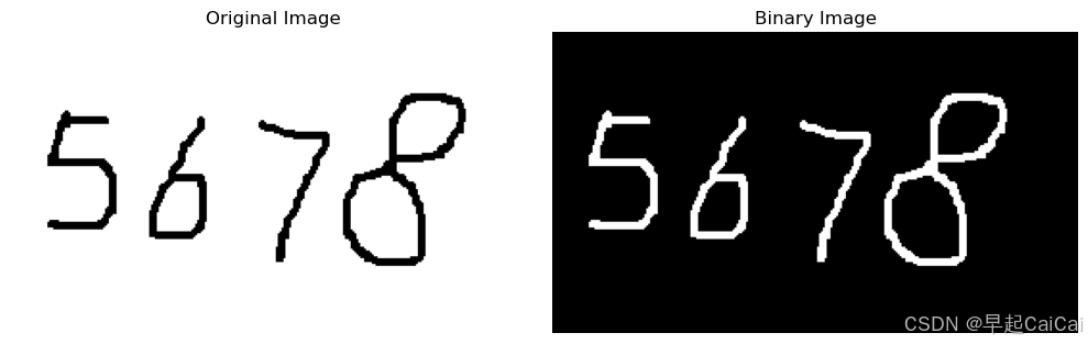
step2 轮廓检测
python
"""
cv2.RETR_EXTERNAL:表示只检测外部轮廓,不考虑内部轮廓
cv2.CHAIN_APPROX_SIMPLE:使用简单的链式近似法来表示轮廓。它将多余的点压缩成直线段,只保留轮廓的端点,从而减少计算量。
"""
contours, _ = cv2.findContours(binary_image, cv2.RETR_EXTERNAL, cv2.CHAIN_APPROX_NONE)
# 按轮廓的中心点的 x 坐标排序
def sort_contours(contours):
    # 将轮廓转换为列表
    contours_list = list(contours)
    # 按 x 坐标排序
    contours_list.sort(key=lambda c: cv2.boundingRect(c)[0])
    return contours_list

# 对轮廓进行排序
contours = sort_contours(contours)
step3 图形切割
python
# 遍历轮廓,提取每个数字
digit_images = []
for contour in contours:
    x, y, w, h = cv2.boundingRect(contour) # cv2.boundingRect(contour):这个函数返回一个最小矩形(bounding box),它包围了每个轮廓
    if h > 20 and w > 10:  # 筛选掉过小的区域
        # digit = binary_image[y:y+h, x:x+w]
        padding = 30  # 增加边缘填充
        digit = binary_image[max(y - padding, 0):y + h + padding, max(x - padding, 0):x + w + padding]
        # digit_resized = cv2.resize(digit, (28, 28))  # 调整到模型输入大小
        digit_images.append(digit)
len(digit_images)
python
plt.figure()
for i in range(len(digit_images)):
    plt.subplot(1, len(digit_images), i + 1)
    plt.tight_layout()
    plt.imshow(digit_images[i], cmap='gray', interpolation='none')
    plt.xticks([])
    plt.yticks([])
plt.show()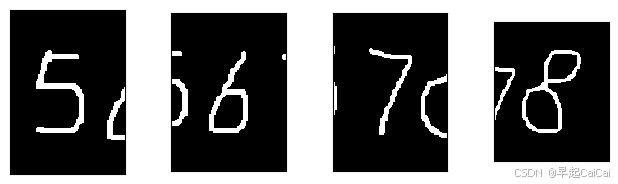
step4 数字识别
python
import torch
from PIL import Image
import torchvision.transforms as transforms

device = torch.device("cuda" if torch.cuda.is_available() else "cpu")
device
python
class Net(torch.nn.Module):
    def __init__(self):
        # (batch,1,28,28)
        super(Net, self).__init__()
        self.conv1 = torch.nn.Sequential(
            torch.nn.Conv2d(1, 32, kernel_size=3), #(batch,32,26,26) 输入通道数1输出通道数32 32为小型任务的经验性选择,一般每层增加一倍欠拟合就加过拟合减
            torch.nn.BatchNorm2d(32), # 对卷积层的输出进行批量归一化,使得每个特征图的分布更加稳定,从而加速训练并提高模型性能。
            torch.nn.ReLU(),
            torch.nn.MaxPool2d(kernel_size=2), #(batch,32,13,13)
        )
        self.conv2 = torch.nn.Sequential(
            torch.nn.Conv2d(32, 64, kernel_size=3), #(batch,64,11,11)
            torch.nn.BatchNorm2d(64),
            torch.nn.ReLU(),
            torch.nn.MaxPool2d(kernel_size=2), #(batch,64,5,5)
        )
        self.fc = torch.nn.Sequential(
            torch.nn.Linear(1600, 50), # 1600 == 64*5*5
            torch.nn.ReLU(),  # 添加ReLU激活函数 增加模型的非线性能力
            torch.nn.Dropout(0.5), # 有效防止过拟合-丢弃率0.5          BN层和dropout层一起用效果不好( 深层可能不好BN在后Dropout在前也不好
            torch.nn.Linear(50, 10)
        )

    def forward(self, x):
        batch_size = x.size(0)
        x = self.conv1(x)  # 一层卷积层,一层池化层,一层激活层
        x = self.conv2(x)  # 再来一次
        x = x.view(batch_size, -1)  # flatten 变成全连接网络需要的输入
        x = self.fc(x)
        return x  # 最后输出的是维度为10的,也就是(对应数学符号的0~9)
python
model = Net().to(device)

model_path = './models/1_Handwritten_Digit_Recognition/model_weights.pth'

# 加载模型参数
model.load_state_dict(torch.load(model_path, map_location=device))

# 将模型设置为评估模式
model.eval()
python
# 预测函数
def predict_image(image, model):
    # image = Image.open(image_path)
    image = Image.fromarray(image)
    # 图像预处理
    transform = transforms.Compose([
        transforms.Grayscale(num_output_channels=1),  # 转换为灰度
        transforms.Resize((28, 28)),                 # 调整到 28x28
        transforms.ToTensor(),                       # 转换为张量
        transforms.Normalize((0.1307,), (0.3081,))         # 归一化到 [-1, 1]
    ])
    image = transform(image)
    image = image.to(device)
    image = image.unsqueeze(0)

    with torch.no_grad():
        output = model(image)
        _, predicted = torch.max(output.data, 1)
    return str(predicted.item())
python
#展示图片
import matplotlib.pyplot as plt
img = Image.open('./data/5678.png')
# 显示图像
plt.imshow(img)
plt.axis('off')  # 可选,关闭坐标轴
plt.show()

predict_digit = []

for image in digit_images:
    predict_digit.append(predict_image(image, model))
print(''.join(predict_digit))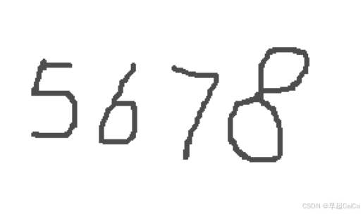
预测结果✅️