文章目录
1.算法原理
去马赛克会在高频区域(尤其是细线条、斜边)产生伪彩色(False Color),表现为边缘处出现彩色条纹。FCS 通过在强边缘区域降低色度(UV)饱和度来抑制假彩色。它的处理逻辑比较简单,如下所示
输入:UV(色度)通道 + edgemap(来自 EE 模块) 下面是实际的FCS算法中,根据最大最小边缘阈值,赋给uv值不同的增益, 强边缘对应弱gain.
if |edgemap| ≤ edge_min:           uvgain = gain        (平坦区域,全保留)
elif edge_min < |edgemap| < edge_max: uvgain = intercept - slope × edgemap  (过渡区,线性衰减)
else:                               uvgain = 0          (强边缘,去色)
2.算法实现
实现细节
- 逐像素处理 UV 两个通道
edge_min和edge_max决定过渡带宽度slope控制过渡带内线性衰减速率
关键参数
| 参数 | 说明 | 典型值 |
|---|---|---|
fcs_edge[0] |
边缘最小阈值 | 32 |
fcs_edge[1] |
边缘最大阈值 | 64 |
gain |
平坦区域 UV 增益(/256) | 32 |
intercept |
线性衰减截距 | 2 |
slope |
线性衰减斜率 | 3 |
算法代码
注:输出中心在 128(对应 UV 中性值),uvgain 控制偏离中心的幅度。
output = uvgain × UV / 256 + 128
python
class FCS:
    'False Color Suppresion'

    def __init__(self, img, edgemap, fcs_edge, gain, intercept, slope):
        self.img = img
        self.edgemap = edgemap
        self.fcs_edge = fcs_edge
        self.gain = gain
        self.intercept = intercept
        self.slope = slope

    def clipping(self):
        np.clip(self.img, 0, 255, out=self.img)
        return self.img

    def execute(self):
        img_h = self.img.shape[0]
        img_w = self.img.shape[1]
        img_c = self.img.shape[2]
        fcs_img = np.empty((img_h, img_w, img_c), np.int16)
        for y in range(img_h):
            for x in range(img_w):
                if np.abs(self.edgemap[y,x]) <= self.fcs_edge[0]:
                    uvgain = self.gain
                elif np.abs(self.edgemap[y,x]) > self.fcs_edge[0] and np.abs(self.edgemap[y,x]) < self.fcs_edge[1]:
                    uvgain = self.intercept - self.slope * self.edgemap[y,x]
                else:
                    uvgain = 0
                fcs_img[y,x,:] = uvgain * (self.img[y,x,:]) / 256 + 128
        self.img = fcs_img
        return self.clipping()
3.测试代码
FCS算法的核心逻辑是根据边缘强度(Edge Map)来动态压低色度(U/V)的增益。下面的例子中,我让千问帮忙生成了一个测试代码,YUV420图像和edgeMap数据. 根据FCS的算法逻辑,UV通道处理逻辑如下
- 第一行(平坦区,Edge=10):由于边缘值小于阈值 32,色彩增益增益为默认gain 32,
- 第二行(过渡区,32 < Edge < 64):边缘值处于过渡区间,算法开始线性衰减色度增益。U/V 值(如 U=180, V=120)被部分压低,向中性值 128 靠近,色彩开始变淡。
- 第三行(强边缘区,Edge=100):由于边缘值大于阈值 64,算法判定此处为强边缘,将色度增益直接置为 0。U/V 值(如 U=240, V=40)被强制拉回 128。
- 第四行(完全平坦区,Edge=0):无边缘,根据算法使用默认gain 32。
python
    def test_fcs_yuv420_visual(self):
        """
        使用 YUV420 格式测试 FCS 算法。
        8x8 的图像对应 4x4 的 U/V 色度通道。
        """
        # 1. 构造 4x4 的模拟真实 UV 数据 (对应 8x8 图像的色度)
        # 第一行: 平坦区,保留鲜艳颜色 (U=200, V=80)
        # 第二行: 过渡区,颜色开始变淡 (U=180, V=120)
        # 第三行: 强边缘区,原本伪彩严重 (U=240, V=40)
        # 第四行: 完全平坦区,正常颜色 (U=160, V=100)
        u_data = np.array([
            [200, 200, 200, 200],
            [180, 180, 180, 180],
            [240, 240, 240, 240],
            [160, 160, 160, 160]
        ], dtype=np.int16)

        v_data = np.array([
            [80, 80, 80, 80],
            [120, 120, 120, 120],
            [40, 40, 40, 40],
            [100, 100, 100, 100]
        ], dtype=np.int16)

        # 组合成 (4, 4, 2) 的 UV 矩阵
        uv = np.stack((u_data, v_data), axis=-1)

        # 2. 构造与色度通道对应的 4x4 edgemap
        edgemap = np.array([
            [10, 10, 10, 10],
            [48, 48, 48, 48],
            [100, 100, 100, 100],
            [0, 0, 0, 0]
        ], dtype=np.int16)

        # 3. 执行 FCS 算法 (此时处理的是 4x4 的色度数据)
        fcs = FCS(uv.copy(), edgemap, fcs_edge=[32, 64], gain=32, intercept=2, slope=3)
        out_uv = fcs.execute()

        # 4. 组装完整的 YUV420 数据以供 OpenCV 转换
        # Y通道设为中性灰 128,尺寸 8x8
        y_channel = np.full((8, 8), 128, dtype=np.uint8)

        # 将处理前后的 UV 通道分离并转为 uint8
        before_u = uv[:, :, 0].astype(np.uint8)
        before_v = uv[:, :, 1].astype(np.uint8)
        after_u = out_uv[:, :, 0].astype(np.uint8)
        after_v = out_uv[:, :, 1].astype(np.uint8)

        # OpenCV 的 YUV420 (I420) 内存布局: [Y (W*H)] + [U (W*H/4)] + [V (W*H/4)]
        before_yuv = np.concatenate([
            y_channel.flatten(),
            before_u.flatten(),
            before_v.flatten()
        ])
        after_yuv = np.concatenate([
            y_channel.flatten(),
            after_u.flatten(),
            after_v.flatten()
        ])

        # 5. 使用 OpenCV 将 YUV420 转换为 BGR (RGB) 以便直观观察
        before_rgb = cv2.cvtColor(before_yuv.reshape((12, 8)), cv2.COLOR_YUV2BGR_I420)
        after_rgb = cv2.cvtColor(after_yuv.reshape((12, 8)), cv2.COLOR_YUV2BGR_I420)

        # 6. 可视化对比 (3x3 布局)
        fig, axes = plt.subplots(3, 3, figsize=(15, 15))

        # 第一行:宏观 RGB 对比
        axes[0, 0].imshow(edgemap, cmap='gray', vmin=0, vmax=100, interpolation='nearest')
        axes[0, 0].set_title('Edge Map (4x4)')

        axes[0, 1].imshow(cv2.cvtColor(before_rgb, cv2.COLOR_BGR2RGB), interpolation='nearest')
        axes[0, 1].set_title('Before FCS (RGB)')

        axes[0, 2].imshow(cv2.cvtColor(after_rgb, cv2.COLOR_BGR2RGB), interpolation='nearest')
        axes[0, 2].set_title('After FCS (RGB)')

        # 第二行:U 通道对比 (4x4)
        axes[1, 0].axis('off')
        axes[1, 1].imshow(before_u, cmap='gray', vmin=0, vmax=255, interpolation='nearest')
        axes[1, 1].set_title('Before FCS - U Channel (4x4)')

        axes[1, 2].imshow(after_u, cmap='gray', vmin=0, vmax=255, interpolation='nearest')
        axes[1, 2].set_title('After FCS - U Channel (4x4)')

        # 第三行:V 通道对比 (4x4)
        axes[2, 0].axis('off')
        axes[2, 1].imshow(before_v, cmap='gray', vmin=0, vmax=255, interpolation='nearest')
        axes[2, 1].set_title('Before FCS - V Channel (4x4)')

        axes[2, 2].imshow(after_v, cmap='gray', vmin=0, vmax=255, interpolation='nearest')
        axes[2, 2].set_title('After FCS - V Channel (4x4)')

        plt.tight_layout()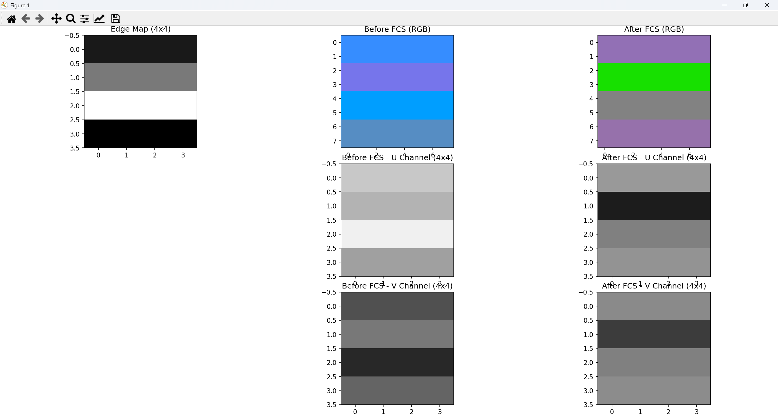
plt.show()- 测试效果图
下图左上角为edgeMap, 这个边缘map数据应该使用EE边缘增强算法生成,但是在实际使用EE算法,报了一些奇怪的问题,考虑到时间关系,最后使用手动构建的的一个map, 这个edgeMap可能不合理,导致RGB前后颜色不match,根据原理,第4行的边缘信息为0,那么它的颜色应该保持一致的,但目前看前后的RGB不太匹配,这中间大概是UV分量改变导致的颜色发生变化.
不过FCS的算法的目的通过在强边缘区域降低色度(UV)饱和度来抑制假彩色