从零手搓大模型（五）把 GPT 微调成垃圾信息分类器

从零手搓大模型第五章教程：把 GPT 微调成垃圾信息分类器

这一章的主题是 Finetuning for Text Classification，也就是"文本分类微调"。

前几章我们做的是：

第 1 章从零手搓大模型（一）文本如何变成 LLM 的输入：文本 -> token ID -> embedding

第 2 章从零手搓大模型（二）Attention 机制到底在算什么：attention 让 token 读取上下文

第 3 章从零手搓大模型（三）从零实现一个 GPT 模型：把 embedding、attention、FFN、LayerNorm 组装成 GPT

第 4 章从零手搓大模型（四）预训练、损失函数与文本生成：真正训练 GPT，让它学会预测下一个 token

第 5 章要做一件很实用的事：

把一个已经预训练好的 GPT，改造成垃圾信息分类器。

也就是说，模型输入一条短信，输出：

not spam（非垃圾信息）
spam（垃圾信息）

1. 本章你要学会什么

学完这一章，你应该能说清楚：

1. classification finetuning 和 instruction finetuning 有什么区别。
2. 为什么要把原始数据集做类别平衡。
3. 为什么文本分类也需要 tokenizer、padding、DataLoader。
4. 如何加载 GPT-2 的预训练权重。
5. 如何把 GPT 的语言模型输出头换成分类输出头。
6. 为什么分类时只取最后一个 token 的输出。
7. 如何计算分类准确率 accuracy。
8. 如何用 cross entropy loss 训练分类器。
9. 为什么只微调最后几层，而不是所有参数。
10. 如何保存和加载微调后的模型。

本章的主线可以压缩成：

短信数据
  -> 清洗和平衡
  -> tokenizer 编码
  -> padding 成同样长度
  -> DataLoader
  -> 加载预训练 GPT
  -> 替换输出头为二分类
  -> 训练分类头和最后几层
  -> 用最后 token 的 logits 判断 spam / not spam

2. 分类微调是什么

微调大模型常见有两种：

1. classification finetuning：分类微调
2. instruction finetuning：指令微调

分类微调的目标是让模型输出一个类别。

比如：

输入：Congratulations! You won a free ticket...
输出：spam

或者：

输入：Can we meet at 5?
输出：not spam

它和第 4 章的预训练不同。

第 4 章预训练时，模型输出的是：

下一个 token 的概率分布

第 5 章分类微调时，模型输出的是：

类别概率

在这个例子里只有两个类别：

0 = ham，也就是 not spam
1 = spam

3. 下载垃圾短信数据集

notebook 使用的是 SMS Spam Collection 数据集。

下载代码如下：

import requests
import zipfile
import os
from pathlib import Path

url = "https://archive.ics.uci.edu/static/public/228/sms+spam+collection.zip"
zip_path = "sms_spam_collection.zip"
extracted_path = "sms_spam_collection"
data_file_path = Path(extracted_path) / "SMSSpamCollection.tsv"

核心下载函数：

def download_and_unzip_spam_data(url, zip_path, extracted_path, data_file_path):
    if data_file_path.exists():
        print(f"{data_file_path} already exists. Skipping download and extraction.")
        return

    response = requests.get(url, stream=True, timeout=60)
    response.raise_for_status()
    with open(zip_path, "wb") as out_file:
        for chunk in response.iter_content(chunk_size=8192):
            if chunk:
                out_file.write(chunk)

    with zipfile.ZipFile(zip_path, "r") as zip_ref:
        zip_ref.extractall(extracted_path)

    original_file_path = Path(extracted_path) / "SMSSpamCollection"
    os.rename(original_file_path, data_file_path)
    print(f"File downloaded and saved as {data_file_path}")

这段代码做了三件事：

1. 如果本地已有数据，就跳过下载。
2. 如果没有，就下载 zip。
3. 解压后把原始文件改名为 .tsv。

.tsv 的意思是 tab-separated values，也就是用制表符分隔的表格文件。

如果SMS Spam Collection 数据集无法下载，这里提SMS Spam Collection 数据集下载地址

链接：https://pan.quark.cn/s/e19b27a5b593

提取码：mbA9

4. 用 pandas 读取数据

import pandas as pd

df = pd.read_csv(data_file_path, sep="\t", header=None, names=["Label", "Text"])
df

输出

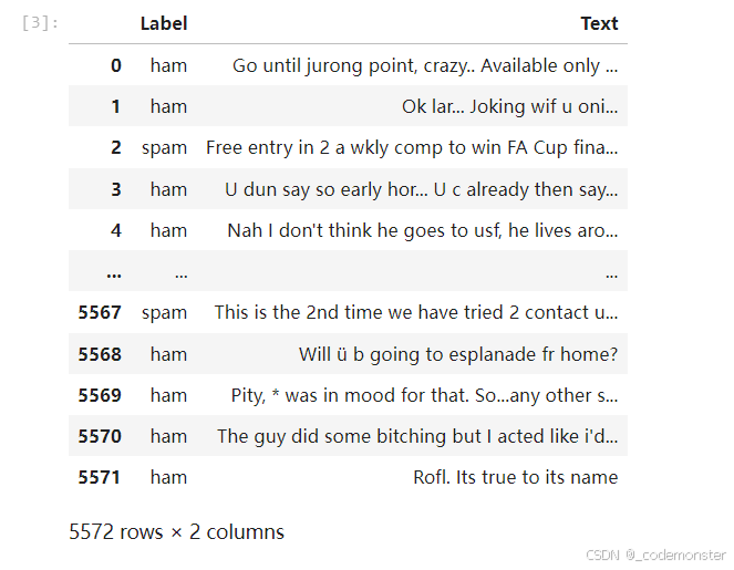
读取后有两列：

Label: ham 或 spam
Text:  内容

其中：

ham  = 正常短信，不是垃圾短信
spam = 垃圾短信

查看类别分布：

print(df["Label"].value_counts())

输出

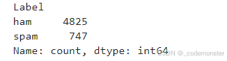
你会发现正常短信比垃圾短信多很多。

这会带来一个问题：如果模型总是预测 ham，准确率也可能看起来不低，但它并没有真正学会识别垃圾短信。

所以做了下面👇类别平衡。

5. 平衡数据集

代码如下：

def create_balanced_dataset(df):

    num_spam = df[df["Label"] == "spam"].shape[0]

    ham_subset = df[df["Label"] == "ham"].sample(num_spam, random_state=123)

    balanced_df = pd.concat([ham_subset, df[df["Label"] == "spam"]])

    return balanced_df


balanced_df = create_balanced_dataset(df)
print(balanced_df["Label"].value_counts())

输出

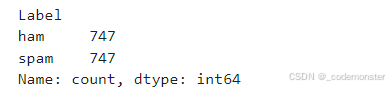
逻辑很简单：

1. 统计 spam 有多少条。
2. 从 ham 里随机抽取同样数量。
3. 把抽出来的 ham 和所有 spam 拼起来。

这样最终数据集里：

ham 数量  = spam 数量

这种做法叫 undersampling，也就是下采样多数类。

优点：

训练更快，类别更平衡，适合教学。

缺点：

丢掉了一部分 ham 数据。

6. 把字符串标签转成数字标签

神经网络不能直接训练字符串标签，所以要转成整数：

balanced_df["Label"] = balanced_df["Label"].map({"ham": 0, "spam": 1})
balanced_df

输出

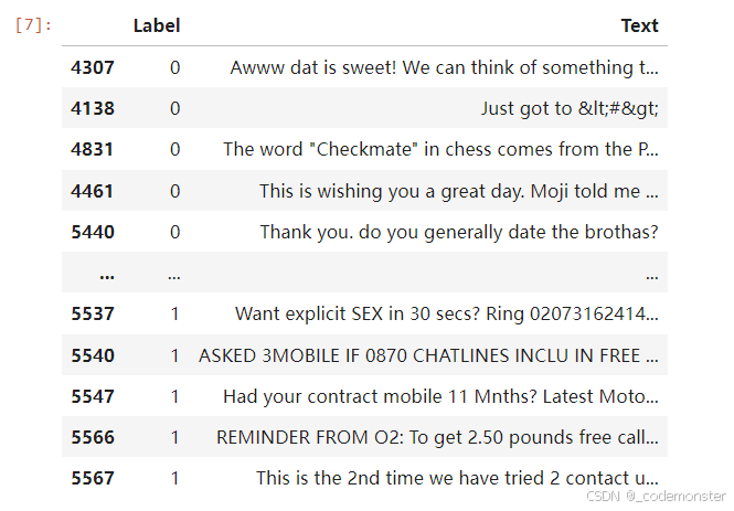
现在：

ham  -> 0
spam -> 1

这正好对应二分类输出：

类别 0：not spam
类别 1：spam

7. 切分训练集、验证集、测试集

代码如下：

def random_split(df, train_frac, validation_frac):
    df = df.sample(frac=1, random_state=123).reset_index(drop=True)

    train_end = int(len(df) * train_frac)
    validation_end = train_end + int(len(df) * validation_frac)

    train_df = df[:train_end]
    validation_df = df[train_end:validation_end]
    test_df = df[validation_end:]

    return train_df, validation_df, test_df


train_df, validation_df, test_df = random_split(balanced_df, 0.7, 0.1)

比例是：

训练集：70%
验证集：10%
测试集：20%

然后保存成 CSV：

train_df.to_csv("train.csv", index=None)
validation_df.to_csv("validation.csv", index=None)
test_df.to_csv("test.csv", index=None)

三者用途不同：

训练集：用来更新模型参数
验证集：训练过程中观察模型表现，辅助调参
测试集：训练完成后做最终评估

8. tokenizer 和 padding

这一章继续使用 GPT-2 tokenizer：

import tiktoken

tokenizer = tiktoken.get_encoding("gpt2")
print(tokenizer.encode("<|endoftext|>", allowed_special={"<|endoftext|>"}))

GPT-2 的 <|endoftext|> token ID 是：

50256

用它作为 padding token。

为什么要 padding

短信长短不一样：

短信 A：3 个 token
短信 B：12 个 token
短信 C：80 个 token

但 DataLoader 要把多条样本组成一个 batch。一个 batch 里的张量必须形状一致。

所以要把短文本补齐到同样长度：

[token1, token2, token3]
-> [token1, token2, token3, pad, pad, pad, ...]

这就是 padding。

9. SpamDataset：把 CSV 变成 PyTorch 数据集

notebook 定义了 SpamDataset：

import torch
from torch.utils.data import Dataset


class SpamDataset(Dataset):
    def __init__(self, csv_file, tokenizer, max_length=None, pad_token_id=50256):
        self.data = pd.read_csv(csv_file)

        self.encoded_texts = [
            tokenizer.encode(text) for text in self.data["Text"]
        ]

        if max_length is None:
            self.max_length = self._longest_encoded_length()
        else:
            self.max_length = max_length
            self.encoded_texts = [
                encoded_text[:self.max_length]
                for encoded_text in self.encoded_texts
            ]

        self.encoded_texts = [
            encoded_text + [pad_token_id] * (self.max_length - len(encoded_text))
            for encoded_text in self.encoded_texts
        ]

    def __getitem__(self, index):
        encoded = self.encoded_texts[index]
        label = self.data.iloc[index]["Label"]
        return (
            torch.tensor(encoded, dtype=torch.long),
            torch.tensor(label, dtype=torch.long)
        )

    def __len__(self):
        return len(self.data)

    def _longest_encoded_length(self):
        max_length = 0
        for encoded_text in self.encoded_texts:
            encoded_length = len(encoded_text)
            if encoded_length > max_length:
                max_length = encoded_length
        return max_length

这个类做了几件事：

1. 读取 CSV。
2. 把每条短信用 tokenizer 编码成 token IDs。
3. 找到最长短信的 token 长度。
4. 把其他短信 padding 到同样长度。
5. 每次返回一个 input tensor 和一个 label tensor。

__getitem__ 返回：

(encoded_text, label)

也就是：

输入 token IDs，目标分类标签

10. 训练集、验证集、测试集的 max_length

训练集这样创建：

train_dataset = SpamDataset(
    csv_file="train.csv",
    max_length=None,
    tokenizer=tokenizer
)

print(train_dataset.max_length)

max_length=None 表示：

自动使用训练集中最长短信的长度。

验证集和测试集则使用同样的 max_length：

val_dataset = SpamDataset(
    csv_file="validation.csv",
    max_length=train_dataset.max_length,
    tokenizer=tokenizer
)

test_dataset = SpamDataset(
    csv_file="test.csv",
    max_length=train_dataset.max_length,
    tokenizer=tokenizer
)

为什么验证集和测试集也用训练集的 max_length？

因为模型训练和评估时输入形状应该一致。

如果验证集或测试集有更长文本，就会被截断：

encoded_text[:self.max_length]

11. 创建 DataLoader

from torch.utils.data import DataLoader

num_workers = 0
batch_size = 8

torch.manual_seed(123)

train_loader = DataLoader(
    dataset=train_dataset,
    batch_size=batch_size,
    shuffle=True,
    num_workers=num_workers,
    drop_last=True,
)

val_loader = DataLoader(
    dataset=val_dataset,
    batch_size=batch_size,
    num_workers=num_workers,
    drop_last=False,
)

test_loader = DataLoader(
    dataset=test_dataset,
    batch_size=batch_size,
    num_workers=num_workers,
    drop_last=False,
)

这里的 batch 大小是 8。

一个 batch 的形状大概是：

input_batch.shape  = (8, max_length)
target_batch.shape = (8,)

含义：

8 条短信，每条短信已经 padding 到 max_length 个 token。

训练集 drop_last=True，是为了确保每个训练 batch 大小一样。

验证集和测试集 drop_last=False，因为评估时不应该丢数据。

12. 加载预训练 GPT-2

本章不是从零训练 GPT，而是加载 GPT-2 small 的预训练权重：

CHOOSE_MODEL = "gpt2-small (124M)"
INPUT_PROMPT = "Every effort moves"

BASE_CONFIG = {
    "vocab_size": 50257,
    "context_length": 1024,
    "drop_rate": 0.0,
    "qkv_bias": True
}

model_configs = {
    "gpt2-small (124M)": {"emb_dim": 768, "n_layers": 12, "n_heads": 12},
    "gpt2-medium (355M)": {"emb_dim": 1024, "n_layers": 24, "n_heads": 16},
    "gpt2-large (774M)": {"emb_dim": 1280, "n_layers": 36, "n_heads": 20},
    "gpt2-xl (1558M)": {"emb_dim": 1600, "n_layers": 48, "n_heads": 25},
}

BASE_CONFIG.update(model_configs[CHOOSE_MODEL])


assert train_dataset.max_length <= BASE_CONFIG["context_length"], (
    f"Dataset length {train_dataset.max_length} exceeds model's context "
    f"length {BASE_CONFIG['context_length']}. Reinitialize data sets with "
    f"`max_length={BASE_CONFIG['context_length']}`"
)

这里选择的是：

gpt2-small
参数量约 124M
embedding 维度 768
Transformer 层数 12
attention heads 12
上下文长度 1024
词表大小 50257

还有一个检查：

assert train_dataset.max_length <= BASE_CONFIG["context_length"]

意思是：

短信 token 长度不能超过模型支持的最大上下文长度。

13. 下载并加载权重

from gpt_download import download_and_load_gpt2
from previous_chapters import GPTModel, load_weights_into_gpt

model_size = CHOOSE_MODEL.split(" ")[-1].lstrip("(").rstrip(")")
settings, params = download_and_load_gpt2(model_size=model_size, models_dir="gpt2")

model = GPTModel(BASE_CONFIG)
load_weights_into_gpt(model, params)
model.eval()

这段代码做了三件事：

1. 下载 GPT-2 权重。
2. 用前面章节实现的 GPTModel 创建模型结构。
3. 把 GPT-2 权重加载进模型。

model.eval() 表示进入推理模式，关闭 dropout 等训练行为。

notebook 还会先让模型生成一小段文本，确认权重加载正常。

14. 为什么原始 GPT 不擅长直接做分类

因为需要用 prompt 让 GPT 判断短信是不是垃圾短信。

但原始 GPT-2 只是预训练语言模型，它学的是：

预测下一个 token

它并没有专门学过：

看到一条短信，输出 spam 或 not spam

所以直接 prompt 的效果不稳定。

这就是为什么要做分类微调。

15. 冻结 GPT 的大部分参数

输出模型

print(model)

输出

GPTModel(
  (tok_emb): Embedding(50257, 768)
  (pos_emb): Embedding(1024, 768)
  (drop_emb): Dropout(p=0.0, inplace=False)
  (trf_blocks): Sequential(
    (0): TransformerBlock(
      (att): MultiHeadAttention(
        (W_query): Linear(in_features=768, out_features=768, bias=True)
        (W_key): Linear(in_features=768, out_features=768, bias=True)
        (W_value): Linear(in_features=768, out_features=768, bias=True)
        (out_proj): Linear(in_features=768, out_features=768, bias=True)
        (dropout): Dropout(p=0.0, inplace=False)
      )
      (ff): FeedForward(
        (layers): Sequential(
          (0): Linear(in_features=768, out_features=3072, bias=True)
          (1): GELU()
          (2): Linear(in_features=3072, out_features=768, bias=True)
        )
      )
      (norm1): LayerNorm()
      (norm2): LayerNorm()
      (drop_resid): Dropout(p=0.0, inplace=False)
    )
    (1): TransformerBlock(
      (att): MultiHeadAttention(
        (W_query): Linear(in_features=768, out_features=768, bias=True)
        (W_key): Linear(in_features=768, out_features=768, bias=True)
        (W_value): Linear(in_features=768, out_features=768, bias=True)
        (out_proj): Linear(in_features=768, out_features=768, bias=True)
        (dropout): Dropout(p=0.0, inplace=False)
      )
      (ff): FeedForward(
        (layers): Sequential(
          (0): Linear(in_features=768, out_features=3072, bias=True)
          (1): GELU()
          (2): Linear(in_features=3072, out_features=768, bias=True)
        )
      )
      (norm1): LayerNorm()
      (norm2): LayerNorm()
      (drop_resid): Dropout(p=0.0, inplace=False)
    )
    (2): TransformerBlock(
      (att): MultiHeadAttention(
        (W_query): Linear(in_features=768, out_features=768, bias=True)
        (W_key): Linear(in_features=768, out_features=768, bias=True)
        (W_value): Linear(in_features=768, out_features=768, bias=True)
        (out_proj): Linear(in_features=768, out_features=768, bias=True)
        (dropout): Dropout(p=0.0, inplace=False)
      )
      (ff): FeedForward(
        (layers): Sequential(
          (0): Linear(in_features=768, out_features=3072, bias=True)
          (1): GELU()
          (2): Linear(in_features=3072, out_features=768, bias=True)
        )
      )
      (norm1): LayerNorm()
      (norm2): LayerNorm()
      (drop_resid): Dropout(p=0.0, inplace=False)
    )
    (3): TransformerBlock(
      (att): MultiHeadAttention(
        (W_query): Linear(in_features=768, out_features=768, bias=True)
        (W_key): Linear(in_features=768, out_features=768, bias=True)
        (W_value): Linear(in_features=768, out_features=768, bias=True)
        (out_proj): Linear(in_features=768, out_features=768, bias=True)
        (dropout): Dropout(p=0.0, inplace=False)
      )
      (ff): FeedForward(
        (layers): Sequential(
          (0): Linear(in_features=768, out_features=3072, bias=True)
          (1): GELU()
          (2): Linear(in_features=3072, out_features=768, bias=True)
        )
      )
      (norm1): LayerNorm()
      (norm2): LayerNorm()
      (drop_resid): Dropout(p=0.0, inplace=False)
    )
    (4): TransformerBlock(
      (att): MultiHeadAttention(
        (W_query): Linear(in_features=768, out_features=768, bias=True)
        (W_key): Linear(in_features=768, out_features=768, bias=True)
        (W_value): Linear(in_features=768, out_features=768, bias=True)
        (out_proj): Linear(in_features=768, out_features=768, bias=True)
        (dropout): Dropout(p=0.0, inplace=False)
      )
      (ff): FeedForward(
        (layers): Sequential(
          (0): Linear(in_features=768, out_features=3072, bias=True)
          (1): GELU()
          (2): Linear(in_features=3072, out_features=768, bias=True)
        )
      )
      (norm1): LayerNorm()
      (norm2): LayerNorm()
      (drop_resid): Dropout(p=0.0, inplace=False)
    )
    (5): TransformerBlock(
      (att): MultiHeadAttention(
        (W_query): Linear(in_features=768, out_features=768, bias=True)
        (W_key): Linear(in_features=768, out_features=768, bias=True)
        (W_value): Linear(in_features=768, out_features=768, bias=True)
        (out_proj): Linear(in_features=768, out_features=768, bias=True)
        (dropout): Dropout(p=0.0, inplace=False)
      )
      (ff): FeedForward(
        (layers): Sequential(
          (0): Linear(in_features=768, out_features=3072, bias=True)
          (1): GELU()
          (2): Linear(in_features=3072, out_features=768, bias=True)
        )
      )
      (norm1): LayerNorm()
      (norm2): LayerNorm()
      (drop_resid): Dropout(p=0.0, inplace=False)
    )
    (6): TransformerBlock(
      (att): MultiHeadAttention(
        (W_query): Linear(in_features=768, out_features=768, bias=True)
        (W_key): Linear(in_features=768, out_features=768, bias=True)
        (W_value): Linear(in_features=768, out_features=768, bias=True)
        (out_proj): Linear(in_features=768, out_features=768, bias=True)
        (dropout): Dropout(p=0.0, inplace=False)
      )
      (ff): FeedForward(
        (layers): Sequential(
          (0): Linear(in_features=768, out_features=3072, bias=True)
          (1): GELU()
          (2): Linear(in_features=3072, out_features=768, bias=True)
        )
      )
      (norm1): LayerNorm()
      (norm2): LayerNorm()
      (drop_resid): Dropout(p=0.0, inplace=False)
    )
    (7): TransformerBlock(
      (att): MultiHeadAttention(
        (W_query): Linear(in_features=768, out_features=768, bias=True)
        (W_key): Linear(in_features=768, out_features=768, bias=True)
        (W_value): Linear(in_features=768, out_features=768, bias=True)
        (out_proj): Linear(in_features=768, out_features=768, bias=True)
        (dropout): Dropout(p=0.0, inplace=False)
      )
      (ff): FeedForward(
        (layers): Sequential(
          (0): Linear(in_features=768, out_features=3072, bias=True)
          (1): GELU()
          (2): Linear(in_features=3072, out_features=768, bias=True)
        )
      )
      (norm1): LayerNorm()
      (norm2): LayerNorm()
      (drop_resid): Dropout(p=0.0, inplace=False)
    )
    (8): TransformerBlock(
      (att): MultiHeadAttention(
        (W_query): Linear(in_features=768, out_features=768, bias=True)
        (W_key): Linear(in_features=768, out_features=768, bias=True)
        (W_value): Linear(in_features=768, out_features=768, bias=True)
        (out_proj): Linear(in_features=768, out_features=768, bias=True)
        (dropout): Dropout(p=0.0, inplace=False)
      )
      (ff): FeedForward(
        (layers): Sequential(
          (0): Linear(in_features=768, out_features=3072, bias=True)
          (1): GELU()
          (2): Linear(in_features=3072, out_features=768, bias=True)
        )
      )
      (norm1): LayerNorm()
      (norm2): LayerNorm()
      (drop_resid): Dropout(p=0.0, inplace=False)
    )
    (9): TransformerBlock(
      (att): MultiHeadAttention(
        (W_query): Linear(in_features=768, out_features=768, bias=True)
        (W_key): Linear(in_features=768, out_features=768, bias=True)
        (W_value): Linear(in_features=768, out_features=768, bias=True)
        (out_proj): Linear(in_features=768, out_features=768, bias=True)
        (dropout): Dropout(p=0.0, inplace=False)
      )
      (ff): FeedForward(
        (layers): Sequential(
          (0): Linear(in_features=768, out_features=3072, bias=True)
          (1): GELU()
          (2): Linear(in_features=3072, out_features=768, bias=True)
        )
      )
      (norm1): LayerNorm()
      (norm2): LayerNorm()
      (drop_resid): Dropout(p=0.0, inplace=False)
    )
    (10): TransformerBlock(
      (att): MultiHeadAttention(
        (W_query): Linear(in_features=768, out_features=768, bias=True)
        (W_key): Linear(in_features=768, out_features=768, bias=True)
        (W_value): Linear(in_features=768, out_features=768, bias=True)
        (out_proj): Linear(in_features=768, out_features=768, bias=True)
        (dropout): Dropout(p=0.0, inplace=False)
      )
      (ff): FeedForward(
        (layers): Sequential(
          (0): Linear(in_features=768, out_features=3072, bias=True)
          (1): GELU()
          (2): Linear(in_features=3072, out_features=768, bias=True)
        )
      )
      (norm1): LayerNorm()
      (norm2): LayerNorm()
      (drop_resid): Dropout(p=0.0, inplace=False)
    )
    (11): TransformerBlock(
      (att): MultiHeadAttention(
        (W_query): Linear(in_features=768, out_features=768, bias=True)
        (W_key): Linear(in_features=768, out_features=768, bias=True)
        (W_value): Linear(in_features=768, out_features=768, bias=True)
        (out_proj): Linear(in_features=768, out_features=768, bias=True)
        (dropout): Dropout(p=0.0, inplace=False)
      )
      (ff): FeedForward(
        (layers): Sequential(
          (0): Linear(in_features=768, out_features=3072, bias=True)
          (1): GELU()
          (2): Linear(in_features=3072, out_features=768, bias=True)
        )
      )
      (norm1): LayerNorm()
      (norm2): LayerNorm()
      (drop_resid): Dropout(p=0.0, inplace=False)
    )
  )
  (final_norm): LayerNorm()
  (out_head): Linear(in_features=768, out_features=50257, bias=False)
)

首先冻结所有参数：

for param in model.parameters():
    param.requires_grad = False

这表示：

训练时不更新这些参数。

为什么要冻结？

因为 GPT-2 已经学到了大量语言知识。我们只想让它适配垃圾短信分类任务，不想从头改动整个模型。

冻结大部分参数有几个好处：

训练更快
显存占用更低
不容易破坏预训练知识
适合小数据集

16. 把语言模型输出头换成分类输出头

原始 GPT 的输出头是：

hidden state -> vocab_size

也就是每个位置输出 50257 个词表 logits，用于预测下一个 token。

分类任务不需要 50257 个输出，只需要 2 个：

not spam
spam

所以替换输出头：

torch.manual_seed(123)

num_classes = 2
model.out_head = torch.nn.Linear(
    in_features=BASE_CONFIG["emb_dim"],
    out_features=num_classes
)

对于 GPT-2 small：

in_features = 768
out_features = 2

现在模型输出变成：

(batch_size, num_tokens, 2)

不是：

(batch_size, num_tokens, 50257)

这是本章最关键的改造。

17. 解冻最后一个 Transformer block 和 final norm

只训练输出头也可以，但效果可能有限。

notebook 还解冻了最后一个 Transformer block 和 final norm：

for param in model.trf_blocks[-1].parameters():
    param.requires_grad = True

for param in model.final_norm.parameters():
    param.requires_grad = True

也就是说，训练时会更新：

1. 新的分类输出头 model.out_head
2. 最后一个 Transformer block
3. final_norm

其余大部分 GPT 参数保持冻结。

这是一种折中：

既利用预训练模型的语言能力，又允许最后几层适配分类任务。

18. 模型输出为什么取最后一个 token

先构造一个输入：

inputs = tokenizer.encode("Do you have time")
inputs = torch.tensor(inputs).unsqueeze(0)
print("Inputs:", inputs)
print("Inputs dimensions:", inputs.shape)

输出

形状是：

(batch_size, num_tokens)

送入模型：

with torch.no_grad():
    outputs = model(inputs)

print("Outputs dimensions:", outputs.shape)

输出

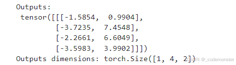
现在输出形状是：

(batch_size, num_tokens, num_classes)

比如：

(1, 4, 2)

每个 token 位置都有一个二分类输出。

那分类时用哪个位置？

使用最后一个 token：

print("Last output token:", outputs[:, -1, :])

输出

为什么用最后一个 token？

因为 GPT 是 causal attention。最后一个 token 可以看到它前面的所有 token。

也就是说：

最后一个 token 的 hidden state 汇聚了整条短信的上下文信息。

所以用最后一个 token 的输出做整条短信的分类。

19. logits、softmax 和 argmax

模型输出的是 logits：

logits = outputs[:, -1, :]

形状：

(batch_size, 2)

可以先转成概率：

probas = torch.softmax(outputs[:, -1, :], dim=-1)
label = torch.argmax(probas)
print("Class label:", label.item())

也可以直接对 logits 做 argmax：

logits = outputs[:, -1, :]
label = torch.argmax(logits)
print("Class label:", label.item())

输出

为什么可以跳过 softmax？

因为 softmax 不改变大小顺序。

logit 最大的类别，softmax 后概率也最大。

所以分类预测时：

predicted_label = argmax(logits)

20. 计算分类准确率

定义

def calc_accuracy_loader(data_loader, model, device, num_batches=None):
    model.eval()
    correct_predictions, num_examples = 0, 0

    if num_batches is None:
        num_batches = len(data_loader)
    else:
        num_batches = min(num_batches, len(data_loader))

    for i, (input_batch, target_batch) in enumerate(data_loader):
        if i < num_batches:
            input_batch, target_batch = input_batch.to(device), target_batch.to(device)

            with torch.no_grad():
                logits = model(input_batch)[:, -1, :]
            predicted_labels = torch.argmax(logits, dim=-1)

            num_examples += predicted_labels.shape[0]
            correct_predictions += (predicted_labels == target_batch).sum().item()
        else:
            break

    return correct_predictions / num_examples

准确率公式：

accuracy = 预测正确数量 / 总样本数量

核心代码是：

predicted_labels = torch.argmax(logits, dim=-1)
correct_predictions += (predicted_labels == target_batch).sum().item()

这里：

predicted_labels: 模型预测类别
target_batch:     真实标签

两者相等就说明预测正确。

21. 分类损失函数：cross entropy

训练时需要 loss。

定义：

def calc_loss_batch(input_batch, target_batch, model, device):
    input_batch, target_batch = input_batch.to(device), target_batch.to(device)
    logits = model(input_batch)[:, -1, :]
    loss = torch.nn.functional.cross_entropy(logits, target_batch)
    return loss

重点是：

torch.nn.functional.cross_entropy(logits, target_batch)

cross entropy 用于分类任务非常常见。

输入：

logits:       (batch_size, num_classes)
target_batch: (batch_size,)

在本章：

num_classes = 2

所以：

logits.shape = (8, 2)
target.shape = (8,)

22. 计算整个 DataLoader 的 loss

def calc_loss_loader(data_loader, model, device, num_batches=None):
    total_loss = 0.

    if len(data_loader) == 0:
        return float("nan")
    elif num_batches is None:
        num_batches = len(data_loader)
    else:
        num_batches = min(num_batches, len(data_loader))

    for i, (input_batch, target_batch) in enumerate(data_loader):
        if i < num_batches:
            loss = calc_loss_batch(input_batch, target_batch, model, device)
            total_loss += loss.item()
        else:
            break

    return total_loss / num_batches

它就是遍历多个 batch，把每个 batch 的 loss 求平均。

num_batches 可以只评估一部分 batch，这样训练过程中评估会更快。

23. 训练函数 train_classifier_simple

训练函数如下：

def train_classifier_simple(model, train_loader, val_loader, optimizer, device, num_epochs,
                            eval_freq, eval_iter):
    train_losses, val_losses, train_accs, val_accs = [], [], [], []
    examples_seen, global_step = 0, -1

    for epoch in range(num_epochs):
        model.train()

        for input_batch, target_batch in train_loader:
            optimizer.zero_grad()
            loss = calc_loss_batch(input_batch, target_batch, model, device)
            loss.backward()
            optimizer.step()
            examples_seen += input_batch.shape[0]
            global_step += 1

            if global_step % eval_freq == 0:
                train_loss, val_loss = evaluate_model(
                    model, train_loader, val_loader, device, eval_iter)
                train_losses.append(train_loss)
                val_losses.append(val_loss)
                print(f"Ep {epoch+1} (Step {global_step:06d}): "
                      f"Train loss {train_loss:.3f}, Val loss {val_loss:.3f}")

        train_accuracy = calc_accuracy_loader(train_loader, model, device, num_batches=eval_iter)
        val_accuracy = calc_accuracy_loader(val_loader, model, device, num_batches=eval_iter)
        print(f"Training accuracy: {train_accuracy*100:.2f}% | ", end="")
        print(f"Validation accuracy: {val_accuracy*100:.2f}%")
        train_accs.append(train_accuracy)
        val_accs.append(val_accuracy)

    return train_losses, val_losses, train_accs, val_accs, examples_seen

训练循环的核心依旧是 PyTorch 标准四步：

optimizer.zero_grad()
loss = calc_loss_batch(...)
loss.backward()
optimizer.step()

含义：

1. 清空上一轮梯度
2. 前向传播并计算 loss
3. 反向传播计算梯度
4. 用优化器更新可训练参数

注意：因为前面冻结了大部分参数，所以真正被更新的主要是：

out_head
最后一个 Transformer block
final_norm

24. evaluate_model

def evaluate_model(model, train_loader, val_loader, device, eval_iter):
    model.eval()
    with torch.no_grad():
        train_loss = calc_loss_loader(train_loader, model, device, num_batches=eval_iter)
        val_loss = calc_loss_loader(val_loader, model, device, num_batches=eval_iter)
    model.train()
    return train_loss, val_loss

评估时要：

model.eval()

并且使用：

with torch.no_grad():

这样可以：

关闭 dropout 等训练行为
不记录梯度，节省内存和计算

评估结束再：

model.train()

切回训练模式。

25. 启动训练

import time

start_time = time.time()

torch.manual_seed(123)

optimizer = torch.optim.AdamW(model.parameters(), lr=5e-5, weight_decay=0.1)

num_epochs = 5
train_losses, val_losses, train_accs, val_accs, examples_seen = train_classifier_simple(
    model, train_loader, val_loader, optimizer, device,
    num_epochs=num_epochs, eval_freq=50, eval_iter=5,
)

end_time = time.time()
execution_time_minutes = (end_time - start_time) / 60
print(f"Training completed in {execution_time_minutes:.2f} minutes.")

输出

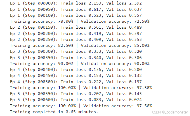
优化器：

AdamW

学习率：

5e-5

训练轮数：

5 epochs

weight_decay=0.1 是一种正则化方式，用来抑制参数过大，减少过拟合。

26. 训练后看什么

画 loss 曲线和 accuracy 曲线。

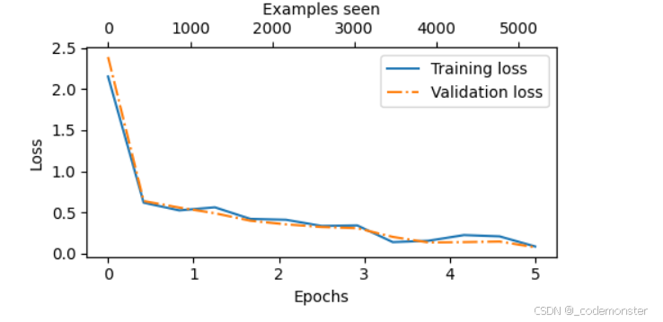
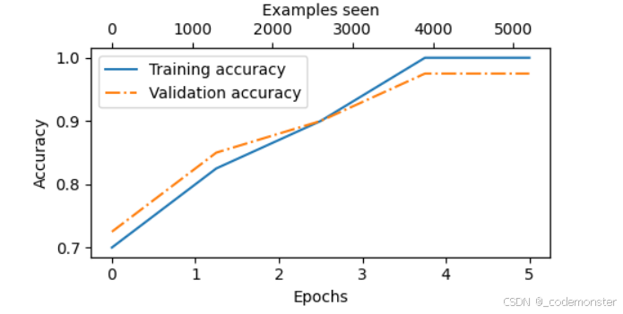
主要看两个趋势：

1. train loss 和 val loss 是否下降。
2. train accuracy 和 val accuracy 是否上升。

如果训练集准确率很高、验证集准确率很低，说明可能过拟合。

如果训练集和验证集都很低，说明模型没学好，可能学习率、训练轮数、数据处理或解冻层数需要调整。

本章正常情况下，微调后准确率会明显提升。

27. 用微调后的模型做分类

定义：

def classify_review(text, model, tokenizer, device, max_length=None, pad_token_id=50256):
    model.eval()

    input_ids = tokenizer.encode(text)
    supported_context_length = model.pos_emb.weight.shape[0]

    input_ids = input_ids[:min(max_length, supported_context_length)]
    assert max_length is not None, (
        "max_length must be specified. If you want to use the full model context, "
        "pass max_length=model.pos_emb.weight.shape[0]."
    )
    assert max_length <= supported_context_length, (
        f"max_length ({max_length}) exceeds model's supported context length ({supported_context_length})."
    )

    input_ids += [pad_token_id] * (max_length - len(input_ids))
    input_tensor = torch.tensor(input_ids, device=device).unsqueeze(0)

    with torch.no_grad():
        logits = model(input_tensor)[:, -1, :]
    predicted_label = torch.argmax(logits, dim=-1).item()

    return "spam" if predicted_label == 1 else "not spam"

函数流程：

1. 输入一条短信文本。
2. tokenizer 编码成 token IDs。
3. 截断到 max_length。
4. padding 到 max_length。
5. 加 batch 维度。
6. 送入模型。
7. 取最后 token 的 logits。
8. argmax 得到类别。
9. 返回 spam 或 not spam。

使用时要传：

max_length=train_dataset.max_length

比如：

print(classify_review(
    "You are a winner you have been specially selected to receive $1000 cash",
    model,
    tokenizer,
    device,
    max_length=train_dataset.max_length
))

输出

虽然函数名叫 classify_review，但这里实际分类的是短信。

28. 保存模型

训练完成后保存权重：

torch.save(model.state_dict(), "review_classifier.pth")

这里保存的是模型参数，不是整个 Python 对象。

这样更推荐，因为更轻量，也更稳定。

29. 加载模型

以后可以这样加载：

model_state_dict = torch.load(
    "review_classifier.pth",
    map_location=device,
    weights_only=True
)
model.load_state_dict(model_state_dict)

注意：加载前需要先创建同样结构的模型。

也就是说，这些步骤要保持一致：

1. 创建 GPTModel(BASE_CONFIG)
2. 加载 GPT-2 预训练权重
3. 替换 out_head 为二分类输出头
4. 再 load_state_dict 加载微调后的权重

30. 本章完整流程回顾

本章可以总结成：

1. 下载 SMS Spam Collection 数据集

2. 读取成 DataFrame
   Label: ham/spam
   Text: 短信内容

3. 类别平衡
   ham 数量 = spam 数量

4. 标签数字化
   ham -> 0
   spam -> 1

5. 切分数据
   train / validation / test

6. tokenizer 编码短信
   text -> token IDs

7. padding 到统一长度
   每个 batch 里的输入形状一致

8. 创建 DataLoader
   input_batch:  (batch_size, max_length)
   target_batch: (batch_size,)

9. 加载 GPT-2 预训练权重

10. 冻结大部分参数

11. 替换输出头
    vocab_size 输出 -> 2 类输出

12. 解冻最后一个 Transformer block 和 final_norm

13. 用最后 token 的 logits 做分类

14. 用 cross entropy loss 训练

15. 用 accuracy 评估

16. 保存微调后的模型

31. 本章最容易混淆的点

为什么输出头从 50257 变成 2

第 4 章做语言建模，需要预测下一个 token，所以输出维度是词表大小：

50257

第 5 章做二分类，只需要输出：

not spam / spam

所以输出维度是：

2

为什么用最后一个 token

GPT 是 causal attention，最后一个 token 能看到前面所有 token。

所以最后位置的输出最适合代表整条短信。

为什么冻结参数

因为我们不是重新训练 GPT，而是在已有语言能力基础上适配一个小分类任务。

冻结参数可以让训练更快，也减少过拟合。

padding token 为什么用 50256

GPT-2 没有专门的 padding token。这里复用 <|endoftext|> 的 token ID：

50256

作为 padding。

为什么验证集和测试集也用训练集 max_length

为了让模型训练、验证、测试时输入长度一致。

如果后续文本太长，就截断；太短，就 padding。

32. 建议

建议按这个顺序学：

1. 先跑数据下载和 df.head()，搞清楚数据长什么样。
2. 跑 create_balanced_dataset，理解为什么要平衡类别。
3. 跑 SpamDataset，重点看 encoded_texts 和 max_length。
4. 跑 DataLoader，确认 batch shape。
5. 跑 GPT-2 加载部分，确认模型能生成文本。
6. 重点看这三段：

for param in model.parameters():
    param.requires_grad = False

model.out_head = torch.nn.Linear(
    in_features=BASE_CONFIG["emb_dim"],
    out_features=2
)

logits = model(input_batch)[:, -1, :]

7. 最后再跑训练函数和分类预测。

如果你只记住本章一句话，记这个：

分类微调就是：保留 GPT 主体，把输出头改成类别输出，再用标注数据训练分类相关参数。

33. 和第 6 章的关系

第 5 章是分类微调，输出是固定类别：

spam / not spam

第 6 章是指令微调，输出是一段自然语言回答：

用户指令 -> 模型回答

所以第 5 章更像传统机器学习分类任务，第 6 章更接近 ChatGPT 这类助手模型的训练方式。

但它们的共同点是：

都不是从零训练模型，而是在预训练 GPT 基础上继续训练。