1.注意力机制
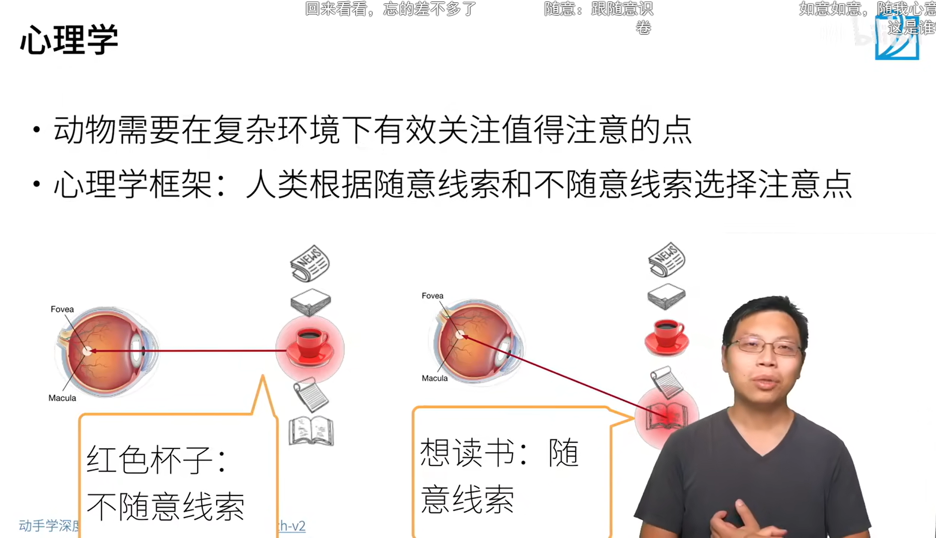
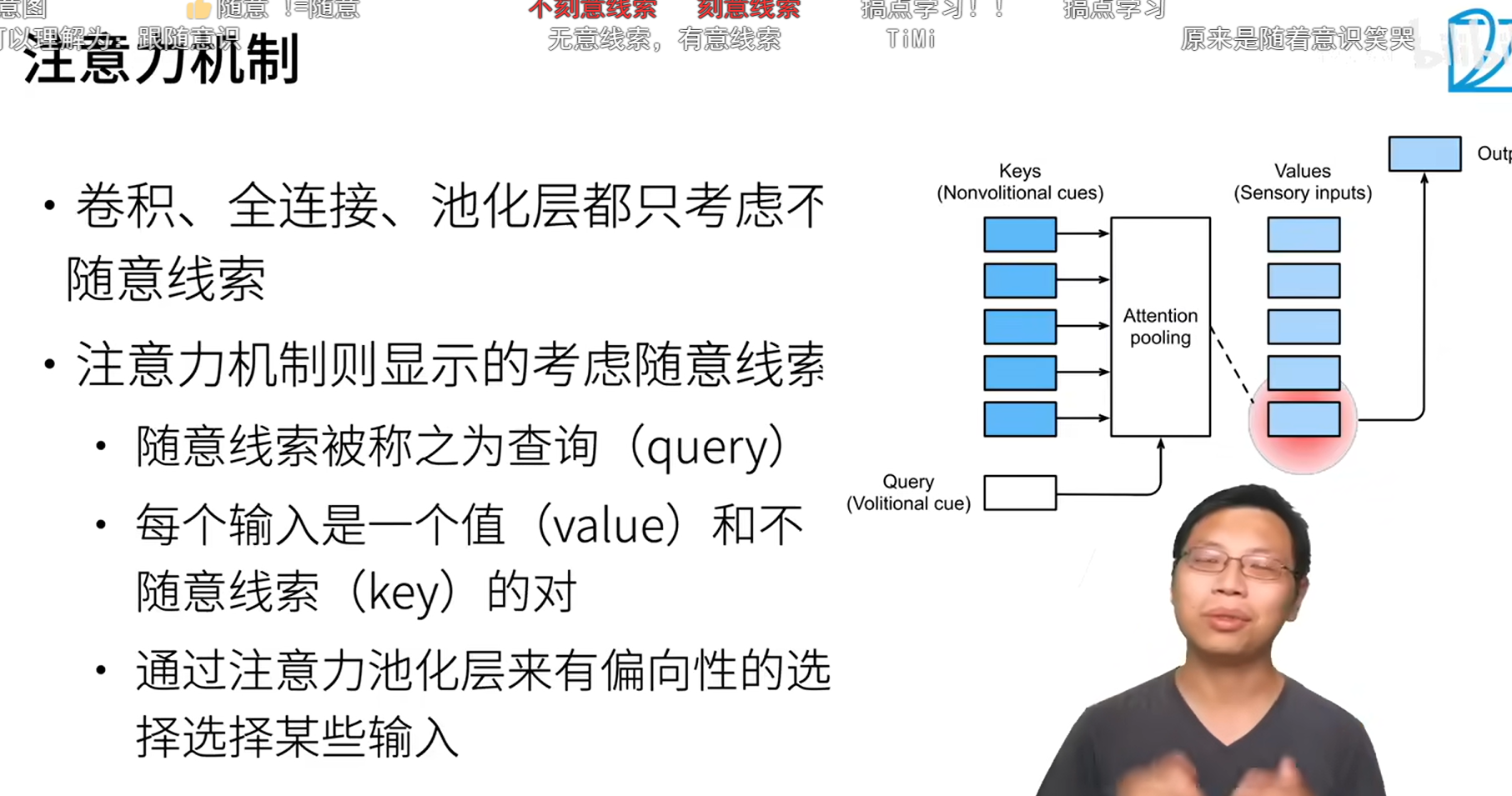
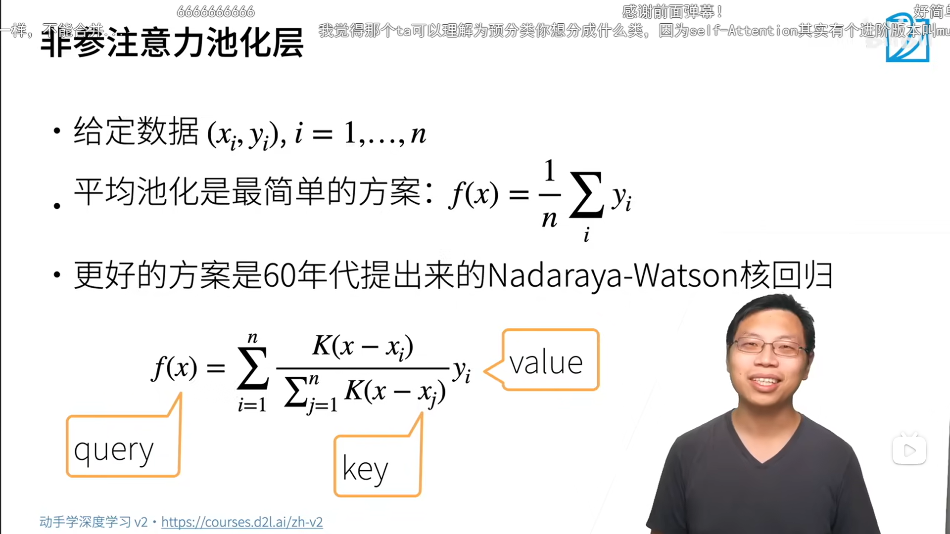
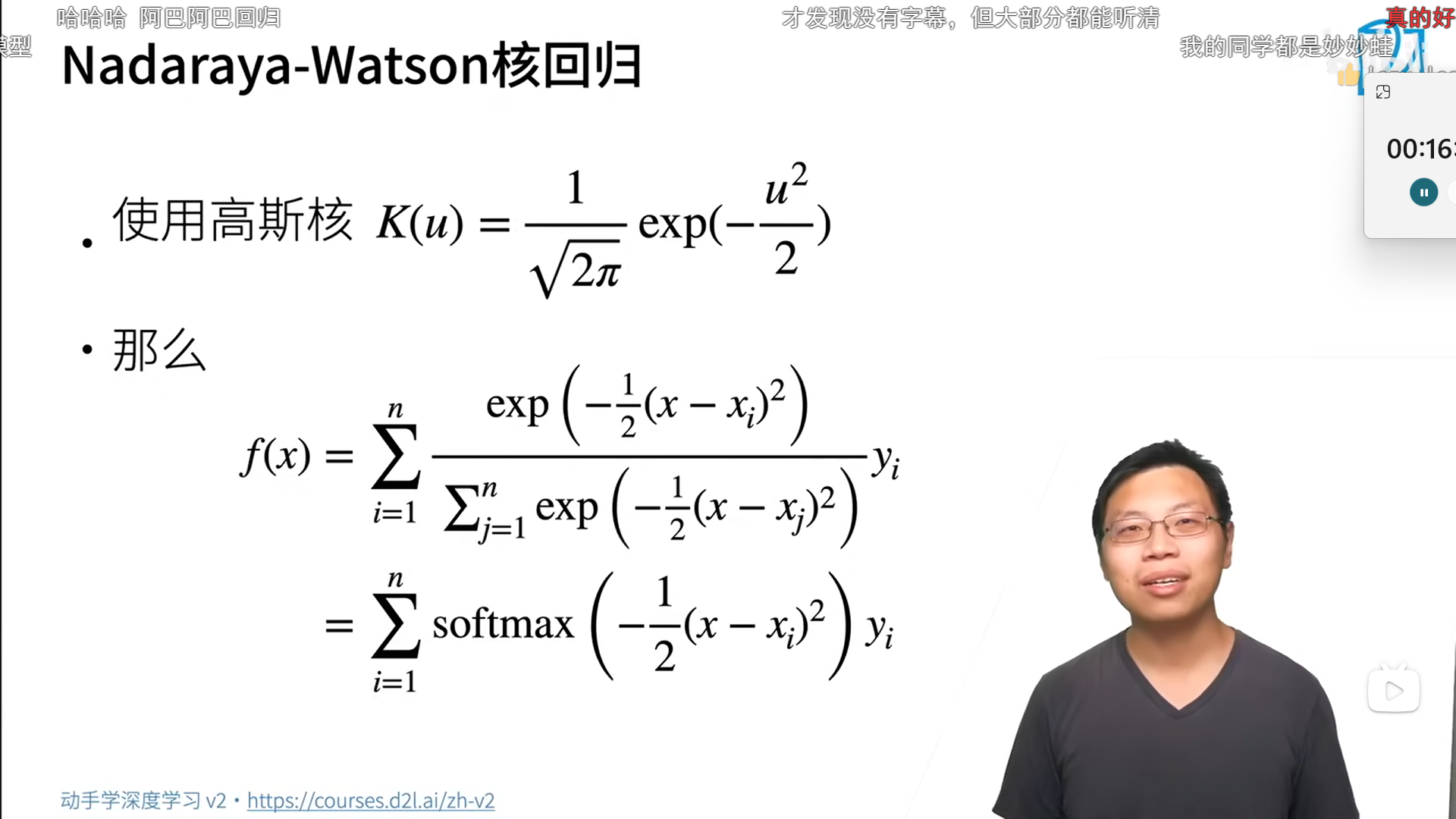
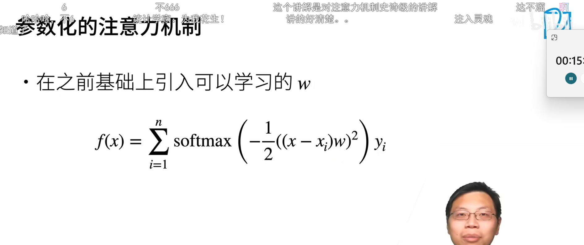
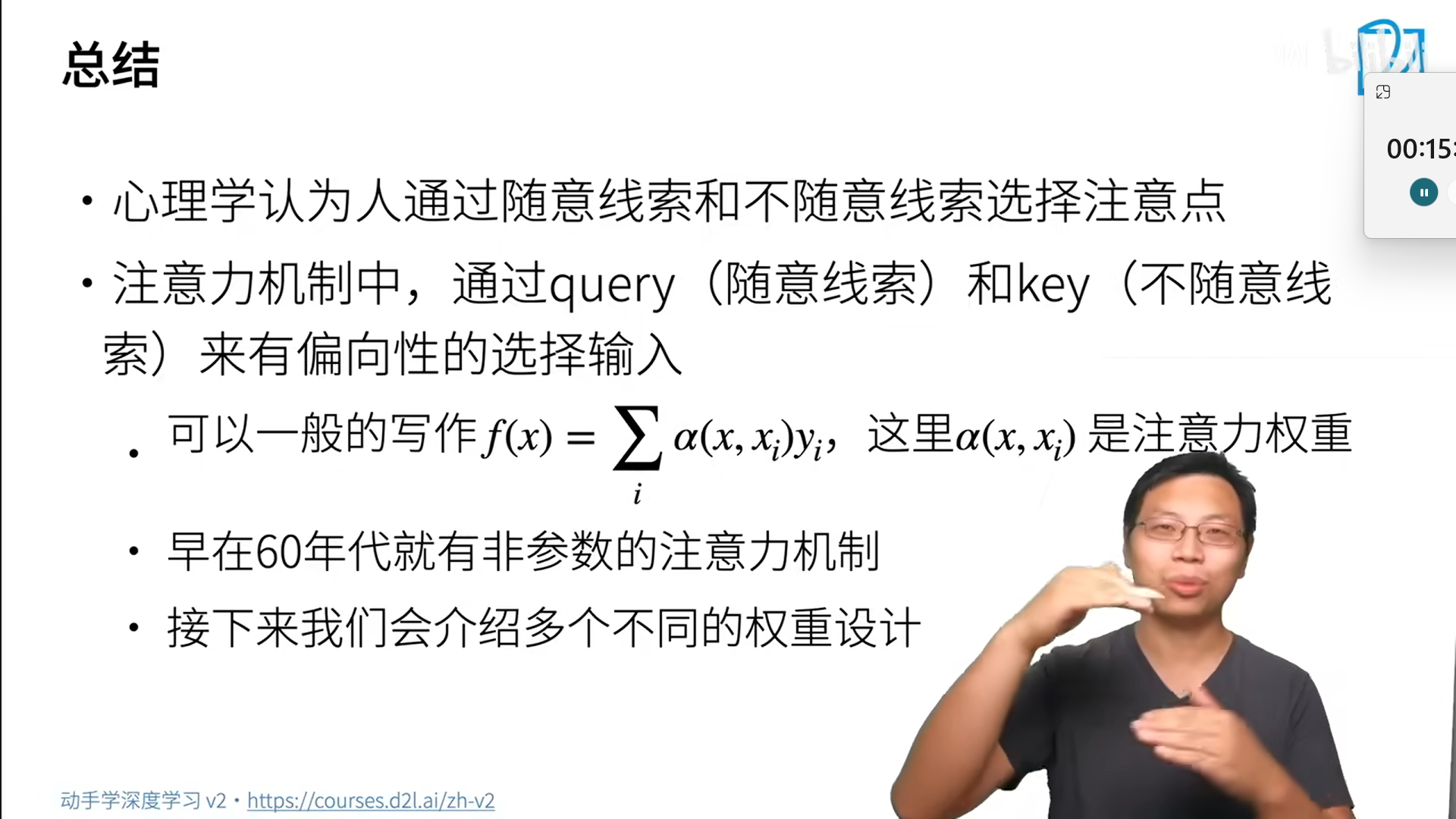
2. 注意力机制
python
import torch
from torch import nn
from d2l import torch as d2l
python
# 生成数据集
# 训练集样本数量
n_train = 50
# 生成训练集特征x_train,范围为[0, 5),并进行排序
x_train, _ = torch.sort(torch.rand(n_train) * 5)
# 定义函数f,用于生成标签y
def f(x):
    return 2 * torch.sin(x) + x**0.8
# 生成训练集标签y_train,并加上服从正态分布的噪声
y_train = f(x_train) + torch.normal(0.0, 0.5, (n_train,))
# 生成测试集特征x_test,范围为[0, 5),步长为0.1
x_test = torch.arange(0, 5, 0.1)
# 生成测试集的真实标签y_truth
y_truth = f(x_test)
# 计算测试集样本数量
n_test = len(x_test)
n_test50
python
# 绘制核回归结果的图像
def plot_kernel_reg(y_hat):
    # 绘制x_test和对应的真实标签y_truth以及预测标签y_hat的图像
    d2l.plot(x_test, [y_truth, y_hat], 'x', 'y', legend=['Truth','Pred'],
            xlim=[0,5], ylim=[-1,5])
    # 绘制训练集的散点图,用圆圈表示
    d2l.plt.plot(x_train, y_train, 'o', alpha=0.5)
# 将y_train的均值重复n_test次作为预测标签y_hat
y_hat = torch.repeat_interleave(y_train.mean(), n_test)
# 调用plot_kernel_reg函数,绘制核回归结果的图像
plot_kernel_reg(y_hat)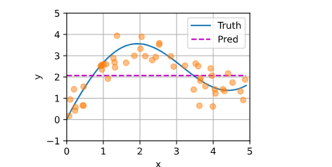
python
# 非参数注意力汇聚
# 将测试集特征x_test重复n_train次并重新reshape为二维矩阵
X_repeat = x_test.repeat_interleave(n_train).reshape((-1, n_train))
# 计算注意力权重,通过对特征差值的平方取负并除以2,再进行softmax归一化
attention_weights = nn.functional.softmax(-(X_repeat - x_train)**2 / 2, dim=1)
# 注意力权重与训练集标签y_train进行矩阵乘法得到预测标签y_hat
y_hat = torch.matmul(attention_weights, y_train)
# 调用plot_kernel_reg函数,绘制非参数注意力汇聚的核回归结果图像
plot_kernel_reg(y_hat)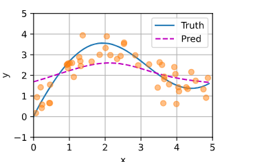
python
# 注意力权重
# 可视化注意力权重
d2l.show_heatmaps(attention_weights.unsqueeze(0).unsqueeze(0),
xlabel='Sorted training inputs', ylabel='Sorted test inputs') 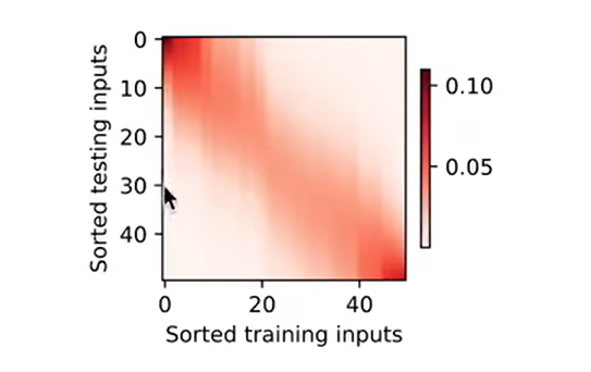
python
# 带参数注意力汇聚
# 假定两个张量的形状分别是(n,a,b)和(n,b,c),它们的批量矩阵乘法输出的形状为(n.a,c)
# 创建形状为(2,1,4)的张量X,元素全为1
X = torch.ones((2,1,4))
# 创建形状为(2,4,6)的张量Y,元素全为1
Y = torch.ones((2,4,6))
# 执行批量矩阵乘法,并输出结果的形状
torch.bmm(X, Y).shapetorch.Size([2, 1, 6])
python
# 使用小批量矩阵乘法来计算小批量数据中的加权平均值
# 创建形状为(2,10)的权重张量,每个权重为0.1
weights = torch.ones((2,10)) * 0.1
# 创建形状为(2,10)的值张量,从0到19的连续数值
values = torch.arange(20.0).reshape((2,10))
# 执行小批量矩阵乘法,计算加权平均值
torch.bmm(weights.unsqueeze(1), values.unsqueeze(-1))tensor([[[ 4.5000]],
[[14.5000]]])
python
# 带参数的注意力汇聚
class NWKernelRegression(nn.Module):
    def __init__(self, **kwargs):
        super().__init__(**kwargs)
        # 创建形状为(1,)的参数张量w,用于调整注意力权重
        self.w = nn.Parameter(torch.rand((1,),requires_grad=True))

    def forward(self, queries, keys, values):
        # 重复queries并调整形状,使其与keys具有相同的列数
        queries = queries.repeat_interleave(keys.shape[1]).reshape(-1,keys.shape[1])
        # 计算注意力权重,通过调整参数w对注意力进行调节
        self.attention_weights = nn.functional.softmax(-((queries - keys) * self.w)**2/2,dim=1)
        # 执行带参数的注意力汇聚,并返回最终结果的形状调整
        return torch.bmm(self.attention_weights.unsqueeze(1),values.unsqueeze(-1)).reshape(-1)
"w"通常指的是权重矩阵,这个矩阵决定了在给定的上下文中,哪些部分应当被赋予更高的关注(即更大的权重)。当我们说"w越窄",我们通常是指权重矩阵的宽度(即列数)较小,这通常对应于较少的关注点或者说更集
python
# 将训练数据集转换为键和值
# 将x_train在行维度上重复n_train次,形成一个矩阵X_tile
X_tile = x_train.repeat((n_train, 1))
# 将y_train在行维度上重复n_train次,形成一个矩阵Y_tile
Y_tile = y_train.repeat((n_train, 1))
# 通过掩码操作,从X_tile中排除对角线元素,得到键矩阵keys
keys = X_tile[(1 - torch.eye(n_train)).type(torch.bool)].reshape((n_train,-1))
# 通过掩码操作,从Y_tile中排除对角线元素,得到值矩阵values
values = Y_tile[(1 - torch.eye(n_train)).type(torch.bool)].reshape(n_train, -1)
python
# 训练带参数的注意力汇聚模型
# 创建带参数的注意力汇聚模型
net = NWKernelRegression()
# 创建均方误差损失函数,用于计算损失
loss = nn.MSELoss(reduction='none')
# 创建随机梯度下降优化器,用于参数更新
trainer = torch.optim.SGD(net.parameters(), lr=0.5)
# 创建动画绘制器,用于绘制损失曲线
animator = d2l.Animator(xlabel='epoch',ylabel='loss',xlim=[1,5])

# 遍历5次
for epoch in range(5):
    # 清零梯度
    trainer.zero_grad()
    # 计算损失
    l = loss(net(x_train, keys, values), y_train) / 2
    # 反向传播,计算梯度
    l.sum().backward()
    # 更新参数
    trainer.step()
    # 打印当前的损失
    print(f'epoch {epoch+1}, loss {float(l.sum()):.6f}')
    # 绘制损失曲线
    animator.add(epoch+1, float(l.sum()))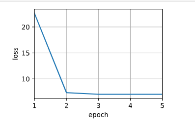
python
# 预测结果绘制
# 将训练数据集的输入在行维度上重复n_test次,形成键矩阵keys
keys = x_train.repeat((n_test, 1))
# 将训练数据集的输出在行维度上重复n_test次,形成值矩阵values
values = y_train.repeat((n_test, 1))
# 使用训练好的模型进行预测,得到预测结果y_hat
y_hat = net(x_test, keys, values).unsqueeze(1).detach()
# 绘制预测结果
plot_kernel_reg(y_hat)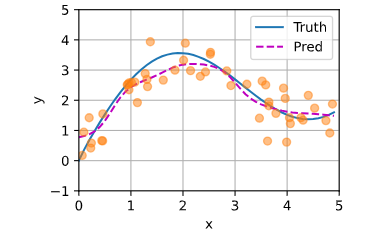
解释:现在是分段拟合,分的段特别多(这个多少是w控制的),所以不平滑
python
# 曲线在注意力权重较大的区域变得更不平滑
d2l.show_heatmaps(net.attention_weights.unsqueeze(0).unsqueeze(0),
xlabel='Sorted training inputs', ylabel='Sorted testing inputs') 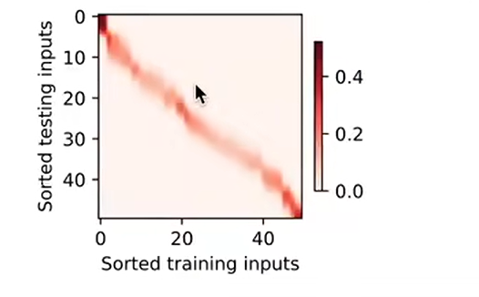
1.注意力分数
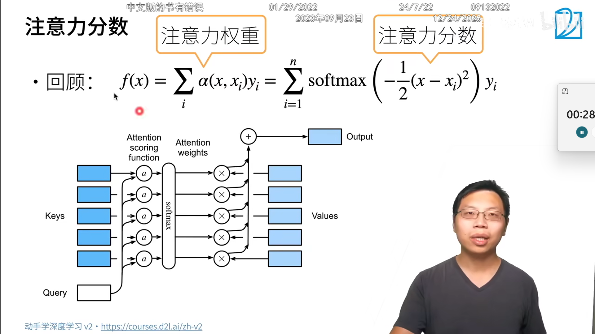
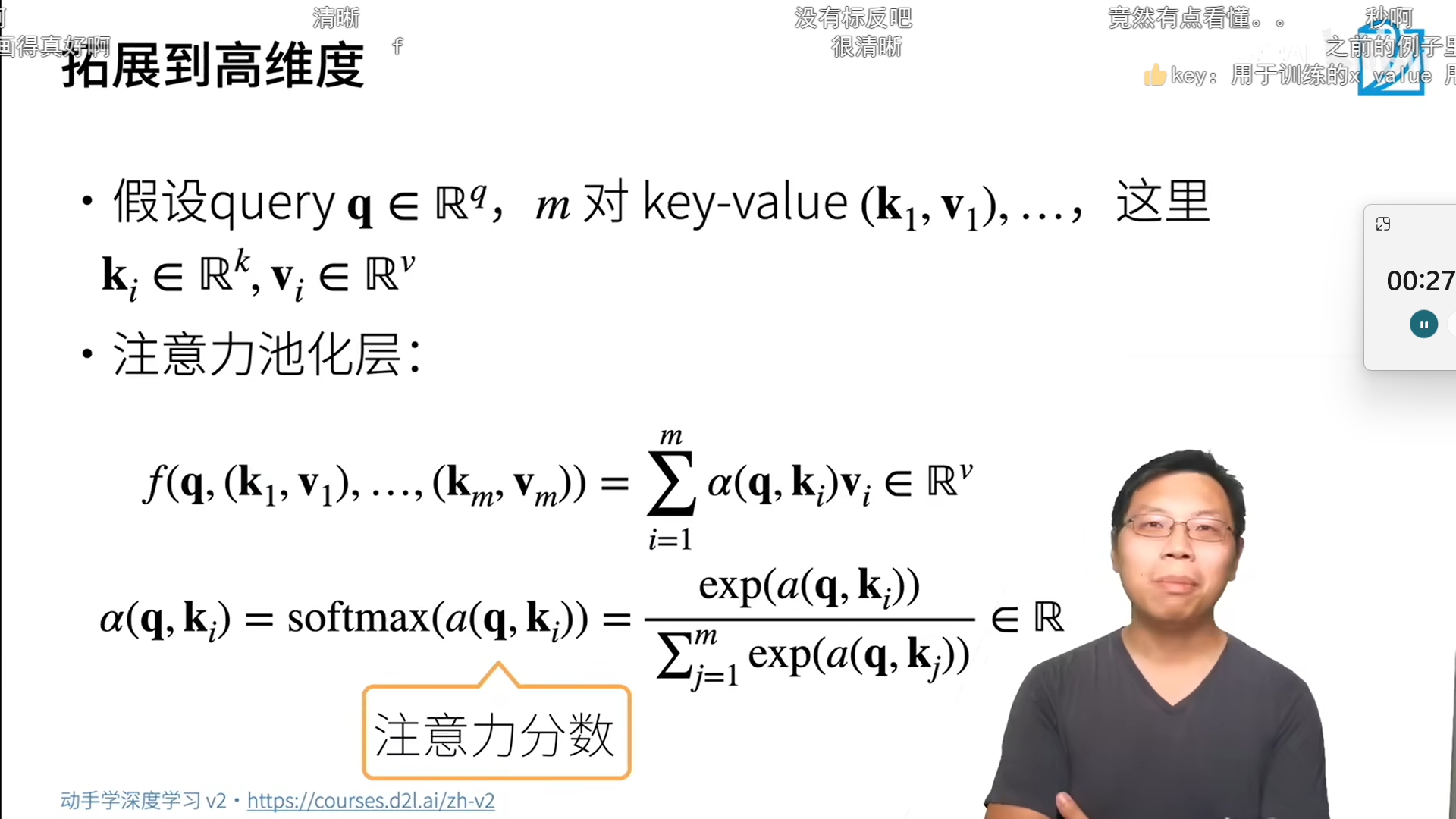
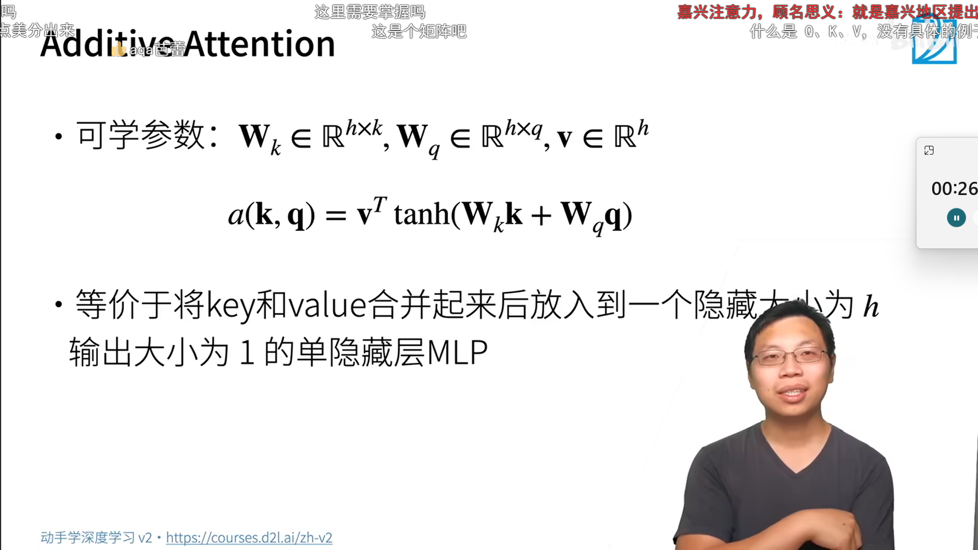
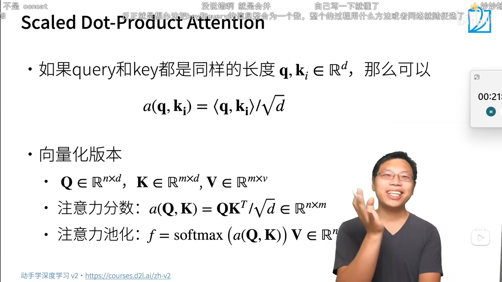
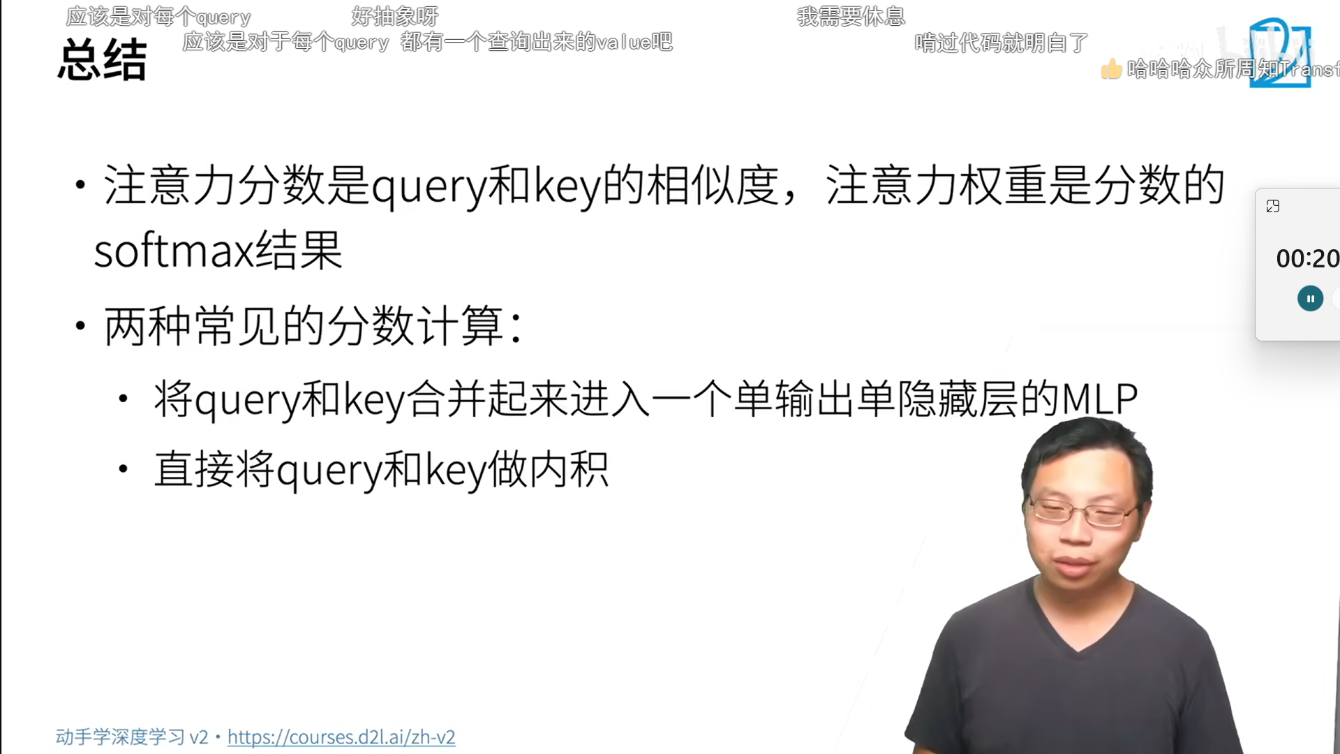
2. 注意力分数
python
import math
import torch
from torch import nn
from d2l import torch as d2l
python
# 遮蔽softmax操作
def masked_softmax(X, valid_lens):
    """通过在最后一个轴上遮蔽元素来执行softmax操作"""
    if valid_lens is None:
        # 如果valid_lens为空,则对X执行softmax操作
        return nn.functional.softmax(X, dim=-1)
    else:
        shape = X.shape
        if valid_lens.dim() == 1:
            # 将valid_lens扩展为与X的最后一个维度相同的形状
            valid_lens = torch.repeat_interleave(valid_lens, shape[1])
        else:
            # 将valid_lens重塑为一维向量
            valid_lens = valid_lens.reshape(-1)
        # 在X的最后一个维度上进行遮蔽操作
        X = d2l.sequence_mask(X.reshape(-1, shape[-1]), valid_lens, value=-1e6)
        # 对遮蔽后的X执行softmax操作,并将形状还原为原始形状
        return nn.functional.softmax(X.reshape(shape), dim=-1)
参考注意力分数矩阵的形状是n*m 相当于一行对应一个query所以是对每行softmax 一些列mask掉舍去没用的填充
python
# 演示此函数是如何工作
# 调用masked_softmax函数,并传入参数
masked_softmax(torch.rand(2,2,4), torch.tensor([2,3]))tensor([[[0.3005, 0.6995, 0.0000, 0.0000],
[0.4543, 0.5457, 0.0000, 0.0000]],
[[0.3104, 0.2572, 0.4324, 0.0000],
[0.2256, 0.3151, 0.4594, 0.0000]]])
python
masked_softmax(torch.rand(2,2,4), torch.tensor([[1,3],[2,4]]))tensor([[[1.0000, 0.0000, 0.0000, 0.0000],
[0.3032, 0.3868, 0.3100, 0.0000]],
[[0.3930, 0.6070, 0.0000, 0.0000],
[0.2379, 0.2396, 0.2583, 0.2642]]])
python
# 加性注意力
class AdditiveAttention(nn.Module):
    """加性注意力"""
    def __init__(self, key_size, query_size, num_hiddens, dropout, **kwargs):
        super(AdditiveAttention, self).__init__(**kwargs)
        # 用于转换键的线性变换
        self.W_k = nn.Linear(key_size, num_hiddens, bias=False)
        # 用于转换查询的线性变换
        self.W_q = nn.Linear(query_size, num_hiddens, bias=False)
        # 用于生成注意力分数的线性变换
        self.w_v = nn.Linear(num_hiddens, 1, bias=False)
        # Dropout层,用于随机丢弃一部分注意力权重
        self.dropout = nn.Dropout(dropout)

    def forward(self, queries, keys, values, valid_lens):
        # 将查询和键进行线性变换
        queries, keys = self.W_q(queries), self.W_k(keys)
        # 执行加性操作,将查询和键相加
        features = queries.unsqueeze(2) + keys.unsqueeze(1)
        # 使用双曲正切函数激活加性操作的结果
        features = torch.tanh(features)
        # 使用线性变换生成注意力分数,并将最后一维的维度压缩掉
        scores = self.w_v(features).squeeze(-1)
        # 使用遮蔽softmax计算注意力权重
        self.attention_weights = masked_softmax(scores, valid_lens)
        # 根据注意力权重对values进行加权求和
        return torch.bmm(self.dropout(self.attention_weights), values)
在使用注意力机制的时候,可以设置bias=False来省略偏置参数。因为注意力机制会根据查询和键之间的相似度来分配权重,而偏置参数可能会干扰这个过程。
python
# 演示上面的AdditiveAttention类
# 创建查询和键张量
queries, keys = torch.normal(0, 1, (2,1,20)), torch.ones((2,10,2))
# 创建值张量
values = torch.arange(40, dtype=torch.float32).reshape(1,10,4).repeat(2,1,1)
# 创建有效长度张量
valid_lens = torch.tensor([2,6])
# 创建加性注意力对象
attention = AdditiveAttention(key_size=2, query_size=20, num_hiddens=8, dropout=0.1)
# 设置为评估模式,不使用dropout
attention.eval()
# 调用加性注意力对象的forward方法
attention(queries, keys, values, valid_lens)tensor([[[ 2.0000, 3.0000, 4.0000, 5.0000]],
[[10.0000, 11.0000, 12.0000, 13.0000]]], grad_fn=<BmmBackward0>)
python
# 注意力权重
# 调用d2l.show_heatmaps函数,显示注意力权重的热图
d2l.show_heatmaps(attention.attention_weights.reshape((1,1,2,10)),
                 xlabel='Keys', ylabel='Queries')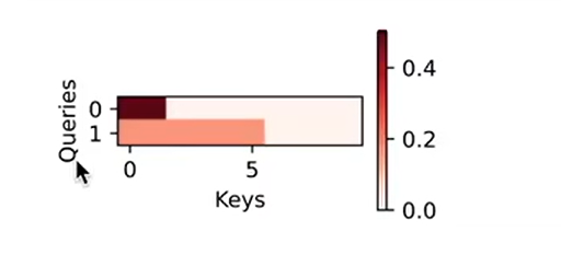
python
# 缩放点积注意力
class DotProductAttention(nn.Module):
    """缩放点积注意力"""
    def __init__(self, dropout, **kwargs):
        super(DotProductAttention, self).__init__(**kwargs)
        # Dropout层,用于随机丢弃一部分注意力权重
        self.dropout = nn.Dropout(dropout)

    def forward(self, queries, keys, values, valid_lens=None):
        # 获取查询向量的维度d
        d = queries.shape[-1]
        # 计算点积注意力得分,并进行缩放
        scores = torch.bmm(queries, keys.transpose(1,2)) / math.sqrt(d)
        # 使用遮蔽softmax计算注意力权重
        self.attention_weights = masked_softmax(scores, valid_lens)
        # 根据注意力权重对values进行加权求和
        return torch.bmm(self.dropout(self.attention_weights), values)
python
# 演示上述的DotProductAttention类
# 创建查询张量
queries = torch.normal(0,1,(2,1,2))
# 创建缩放点积注意力对象
attention = DotProductAttention(dropout=0.5)
# 设置为评估模式,不使用dropout
attention.eval()
# 调用缩放点积注意力对象的forward方法
attention(queries, keys, values, valid_lens)tensor([[[ 2.0000, 3.0000, 4.0000, 5.0000]],
[[10.0000, 11.0000, 12.0000, 13.0000]]])
python
# 均匀的注意力权重
# 调用d2l.show_heatmaps函数,显示注意力权重的热图
d2l.show_heatmaps(attention.attention_weights.reshape((1,1,2,10)),
                 xlabel='Keys', ylabel='Queries')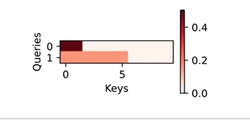
1. 使用注意力机制的seq2seq
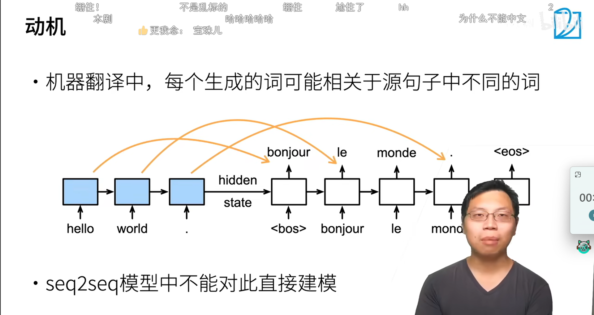
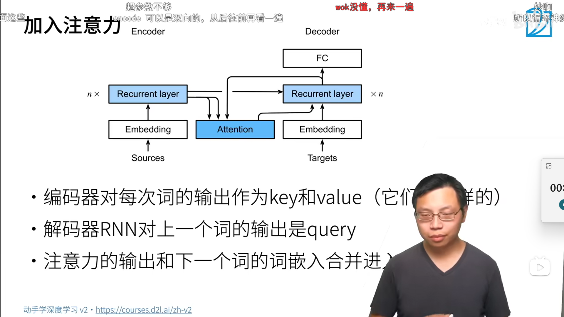
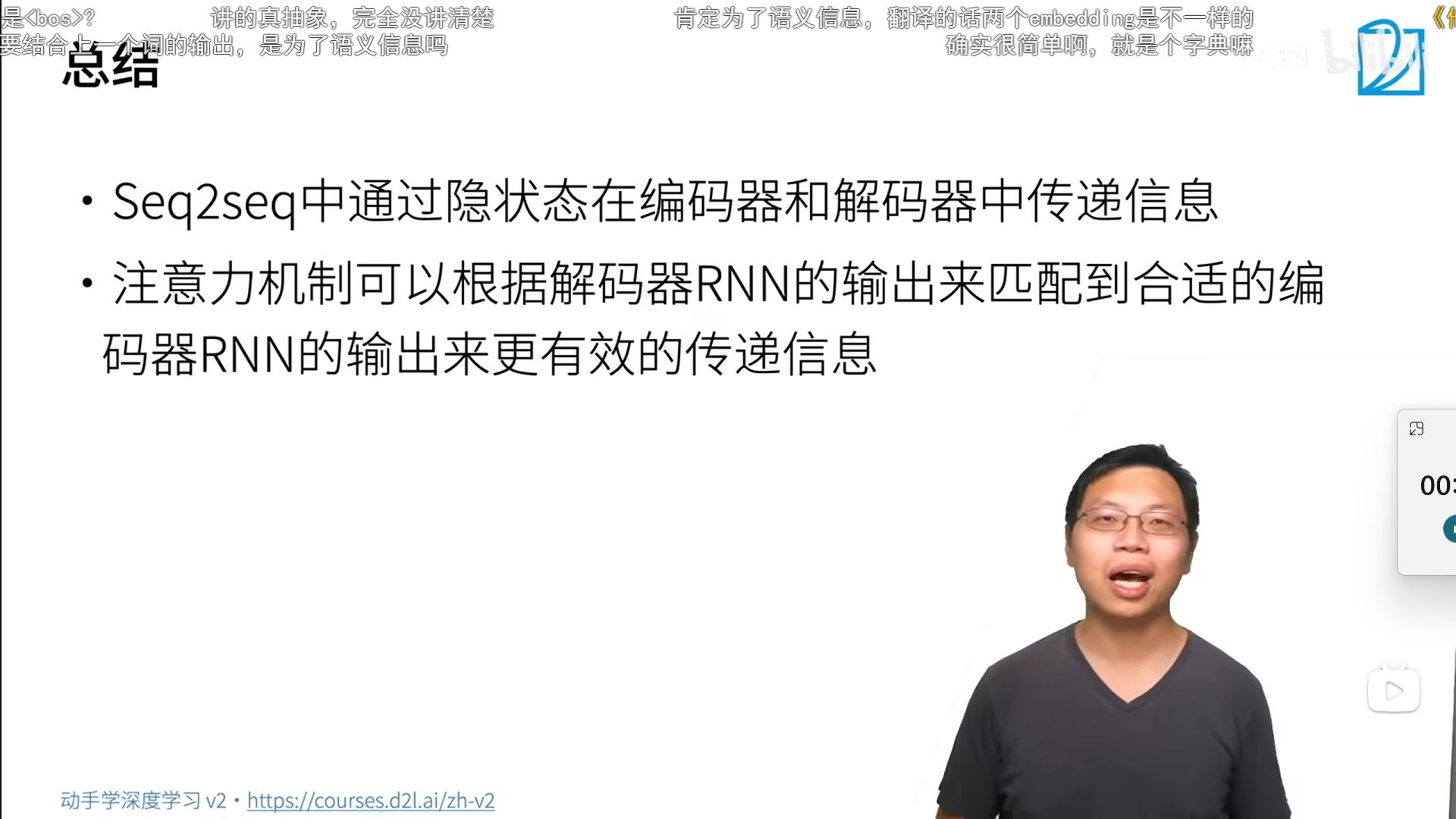
2. 使用注意力机制的seq2seq
python
import torch
from torch import nn
from d2l import torch as d2l
import os
python
# 带有注意力机制的解码器基本接口
class AttentionDecoder(d2l.Decoder):
    """带有注意力机制的解码器基本接口"""
    def __init__(self, **kwargs):
        super(AttentionDecoder, self).__init__(**kwargs)

    @property
    def attention_weight(self):
        raise NotImplementedError
python
# 实现带有Bahdanau注意力的循环神经网络解码器
class Seq2SeqAttentionDecoder(AttentionDecoder):
    def __init__(self, vocab_size, embed_size, num_hiddens, num_layers, dropout=0, **kwargs):
        # 调用父类AttentionDecoder的构造函数进行初始化
        super(Seq2SeqAttentionDecoder, self).__init__(**kwargs)
        # 创建一个加性注意力机制的实例,用于计算注意力权重
        self.attention = d2l.AdditiveAttention(num_hiddens, num_hiddens, num_hiddens, dropout)
        # 创建一个嵌入层,用于将输入的整数序列进行嵌入表示
        self.embedding = nn.Embedding(vocab_size, embed_size)
        # 创建一个GRU层,用于实现循环神经网络的计算
        self.rnn = nn.GRU(embed_size + num_hiddens, num_hiddens, num_layers, dropout=dropout)
        # 创建一个线性层,将隐藏状态映射到词汇表大小的输出
        self.dense = nn.Linear(num_hiddens, vocab_size)

    def init_state(self, enc_outputs, enc_valid_lens, *args):
        # 将编码器的输出解包为outputs和hidden_state
        outputs, hidden_state = enc_outputs
        # 对outputs进行维度变换,将batch维和时间步维交换,保持与解码器输入的一致性
        # 返回初始化的解码器隐藏状态
        return (outputs.permute(1, 0, 2), hidden_state, enc_valid_lens)

    def forward(self, X, state):
        # 解析输入的状态信息,包括编码器的输出、隐藏状态和有效长度
        enc_outputs, hidden_state, enc_valid_lens = state
        # 对输入序列进行嵌入表示,并进行维度变换,将batch维和时间步维交换
        X = self.embedding(X).permute(1, 0, 2)
        # 初始化输出列表和注意力权重列表
        outputs, self._attention_weights = [], []
        for x in X:
            # 获取当前时间步的查询向量,将隐藏状态的最后一个时间步的特征进行维度扩展
            query = torch.unsqueeze(hidden_state[-1], dim=1)
            # 计算注意力上下文向量,通过注意力机制对编码器的输出进行加权求和
            context = self.attention(query, enc_outputs, enc_outputs, enc_valid_lens)
            # 将注意力上下文向量与当前时间步的输入进行拼接,用于输入到循环神经网络
            x = torch.cat((context, torch.unsqueeze(x, dim=1)), dim=-1)
            # 执行循环神经网络的前向计算,得到输出和更新后的隐藏状态
            out, hidden_state = self.rnn(x.permute(1,0,2),hidden_state)
            # 将输出和注意力权重添加到对应的列表中
            outputs.append(out)
            self._attention_weights.append(self.attention.attention_weights)
        # 将输出列表中的结果进行拼接,并通过线性层进行映射
        outputs = self.dense(torch.cat(outputs, dim=0))
        # 对输出进行维度变换,将batch维和时间步维交换,并返回更新后的状态信息
        return outputs.permute(1, 0, 2), [enc_outputs, hidden_state, enc_valid_lens]

    @property
    def attention_weights(self):
        # 返回注意力权重
        return self._attention_weights
python
# 测试Bahdanau注意力解码器
# 创建编码器和解码器的实例
encoder = d2l.Seq2SeqEncoder(vocab_size = 10, embed_size=8, num_hiddens=16, num_layers=2)
encoder.eval()
decoder = Seq2SeqAttentionDecoder(vocab_size=10, embed_size=8, num_hiddens=16,num_layers=2)
decoder.eval()
# 创建输入序列X
X = torch.zeros((4,7), dtype=torch.long)
# 初始化解码器的状态
state = decoder.init_state(encoder(X), None)
# 执行解码器的前向计算
output, state = decoder(X, state)
# 输出结果的形状以及状态信息的长度和形状
output.shape, len(state), state[0].shape, len(state[1]), state[1][0].shape(torch.Size([4, 7, 10]), 3, torch.Size([4, 7, 16]), 2, torch.Size([4, 16]))
python
def read_data_nmt():
    """载入 "英语-法语" 数据集 """
    # 下载并解压数据集
    data_dir = d2l.download_extract('fra-eng')
    # 打开数据文件,使用utf-8编码读取文件内容
    with open(os.path.join(data_dir, 'fra.txt'), 'r', encoding='utf-8') as f:
        # 返回读取的文件内容
        return f.read()
python
def preprocess_nmt(text):
    """预处理 "英语-法语" 数据集"""
    def no_space(char, prev_char):
        # 检查是否需要在字符之前添加空格
        return char in set(',.!?') and prev_char != ''
    # 替换特殊字符为空格并转换为小写
    text = text.replace('\u202f', ' ').replace('\xa0',' ').lower()
    # 根据规则在字符之前添加空格
    out = [
        ' ' + char if i > 0 and no_space(char, text[i - 1]) else char
        for i, char in enumerate(text)]
    # 将处理后的字符列表连接成字符串并返回
    return ''.join(out)
python
def tokenize_nmt(text, num_examples=None):
    """词元化 "英语-法语" 数据数据集 """
    # 初始化源语言和目标语言的列表
    source, target = [], []
    # 对每行文本进行遍历
    for i, line in enumerate(text.split('\n')):
        # 如果指定了num_examples,并且超过了指定数量,则退出循环
        if num_examples and i > num_examples:
            break
        # 将每行文本按制表符分割成源语言和目标语言的部分
        parts = line.split('\t')
        # 如果分割后有两个部分,说明包含了源语言和目标语言的内容
        if len(parts) == 2:
            # 将源语言部分以空格为分隔符进行词元化,存储到源语言列表中
            source.append(parts[0].split(' '))
            # 将目标语言部分以空格为分隔符进行词元化,存储到目标语言列表中
            target.append(parts[1].split(' '))
    # 返回词元化后的源语言列表和目标语言列表
    return source, target
python
def truncate_pad(line, num_steps, padding_token):
    """截断或填充文本序列"""
    # 如果文本序列的长度超过了指定的步数
    if len(line) > num_steps:
        # 截断文本序列,保留前num_steps个元素
        return line[:num_steps]
    # 在文本序列末尾填充padding_token,使其长度达到num_steps
    return line + [padding_token] * (num_steps - len(line))
python
def build_array_nmt(lines, vocab, num_steps):
    """将机器翻译的文本序列转换成小批量"""
    # 将文本序列中的每个词根据词汇表转换为对应的索引
    lines = [vocab[l] for l in lines]
    # 在每个文本序列末尾添加<eos>表示句子结束的索引
    lines = [l + [vocab['<eos>']] for l in lines]
    # 将每个文本序列截断或填充为固定长度,并转换为tensor形式
    array = torch.tensor([ truncate_pad(l, num_steps, vocab['<pad>']) for l in lines ])
    # 计算有效长度,即非填充部分的长度
    valid_len = (array != vocab['<pad>']).type(torch.int32).sum(1)
    # 返回转换后的tensor形式的文本序列和有效长度
    return array, valid_len
python
def load_data_nmt(batch_size, num_steps, num_examples=600):
    """返回翻译数据集的迭代器和词汇表"""
    # 载入并预处理文本数据集
    text = preprocess_nmt(read_data_nmt())
    # 将文本数据集进行词元化
    source, target = tokenize_nmt(text, num_examples)
    # 构建源语言的词汇表对象
    src_vocab = d2l.Vocab(source, min_freq=2,
                         reserved_tokens=['<pad>','<bos>','<eos>'])
    # 构建目标语言的词汇表对象
    tgt_vocab = d2l.Vocab(target, min_freq=2,
                         reserved_tokens=['<pad>','<bos>','<eos>'])
    # 将源语言文本序列转换为小批量数据,并获取有效长度
    src_array, src_valid_len = build_array_nmt(source, src_vocab, num_steps)
    # 将目标语言文本序列转换为小批量数据,并获取有效长度
    tgt_array, tgt_valid_len = build_array_nmt(target, tgt_vocab, num_steps)
    # 构建数据集的数组
    data_arrays = (src_array, src_valid_len, tgt_array, tgt_valid_len)
    # 构建数据迭代器
    data_iter = d2l.load_array(data_arrays, batch_size)
    # 返回数据迭代器和词汇表对象
    return data_iter, src_vocab, tgt_vocab
python
# 训练
# 设置嵌入大小、隐藏层大小、层数和丢弃率
embed_size, num_hiddens, num_layers, dropout = 32, 32, 2, 0.1
# 设置批量大小和序列长度
batch_size, num_steps = 64, 10
# 设置学习率、训练轮数和设备(GPU或CPU)
lr, num_epochs, device = 0.005, 250, d2l.try_gpu()

# 载入翻译数据集,并获取数据迭代器和词汇表
train_iter, src_vocab, tgt_vocab = load_data_nmt(batch_size, num_steps)
# 创建源语言的编码器实例
encoder = d2l.Seq2SeqEncoder(len(src_vocab), embed_size, num_hiddens, num_layers, dropout)
# 创建目标语言的带有注意力机制的解码器实例
decoder = Seq2SeqAttentionDecoder(len(tgt_vocab), embed_size, num_hiddens, num_layers, dropout)
# 创建编码-解码模型实例
net = d2l.EncoderDecoder(encoder, decoder)
# 训练序列到序列模型
d2l.train_seq2seq(net, train_iter, lr, num_epochs, tgt_vocab, device)loss 0.018, 7276.1 tokens/sec on cuda:0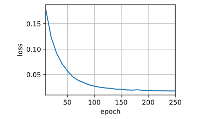
python
# 将几个英语句子翻译成汉语
# 英语句子列表
engs = ['go', "i lost .", 'he\'s calm .', 'i\'m home .']
# 对应的汉语句子列表
fras = ['va !', 'j\' ai perdu .', 'il est calme .', 'je suis chez moi .']
# 遍历英语句子和汉语句子的对应关系
for eng, fra in zip(engs, fras):
    # 使用训练好的模型net对英语句子进行翻译,并获取注意力权重序列
    translation, dec_attention_weight_seq = d2l.predict_seq2seq(net, eng, src_vocab,
                                                               tgt_vocab, num_steps, device, True)
    # 打印英语句子、翻译结果和BLEU分数
    print(f' {eng} => {translation}, ',
f'bleu {d2l.bleu(translation, fra, k=2):.3f}') go => va !, bleu 0.000
i lost . => j'ai perdu ., bleu 0.492
he's calm . => il est malade ., bleu 0.658
i'm home . => je suis chez moi ., bleu 1.000
python
# 将注意力权重序列进行拼接,并调整形状
attention_weights = torch.cat([step[0][0][0] for step in dec_attention_weight_seq], 0).reshape((1, 1, -1, num_steps))
python
# 可视化注意力权重
# 显示注意力权重的热图,仅显示与输入英语句子对应的位置
d2l.show_heatmaps(attention_weights[:,:,:,:len(engs[-1].split()) + 1].cpu(),
                 xlabel = 'key positions', ylabel = 'Query posistions')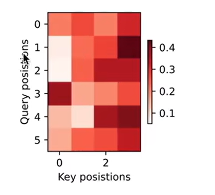
1. 自注意力
2. 自注意力
python
import math
import torch
from torch import nn
from d2l import torch as d2l
python
# 设置隐藏单元数量和头的数量
num_hiddens, num_heads = 100, 5
# 创建多头注意力实例
# 输入参数为隐藏单元数量、查询维度、键维度、值维度、头的数量和dropout率
attention = d2l.MultiHeadAttention(num_hiddens, num_hiddens, num_hiddens,
                                  num_hiddens, num_heads, 0.5)
# 将多头注意力设置为评估模式,不进行训练
attention.eval()MultiHeadAttention(
(attention): DotProductAttention(
(dropout): Dropout(p=0.5, inplace=False)
)
(W_q): Linear(in_features=100, out_features=100, bias=False)
(W_k): Linear(in_features=100, out_features=100, bias=False)
(W_v): Linear(in_features=100, out_features=100, bias=False)
(W_o): Linear(in_features=100, out_features=100, bias=False)
)
python
# 设置批量大小、查询数和有效长度
batch_size, num_queries, valid_lens = 2, 4, torch.tensor([3, 2])
# 创建形状为(batch_size, num_queries, num_hiddens)的输入张量X,初始化为全1
X = torch.ones((batch_size, num_queries, num_hiddens))
# 对输入张量X应用多头注意力机制,并获取输出的形状
attention(X, X, X, valid_lens).shapetorch.Size([2, 4, 100])
python
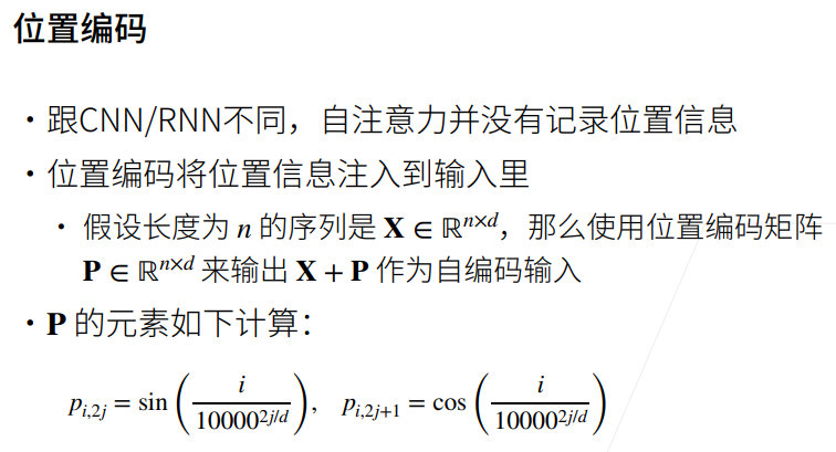
# 位置编码
class PositionalEncoding(nn.Module):
    # 初始化函数,接收隐藏单元数量、dropout率和最大序列长度作为输入
    def __init__(self, num_hiddens, dropout, max_len=1000):
        # 调用父类的初始化函数
        super(PositionalEncoding, self).__init__()
        # 创建一个dropout层,用于随机丢弃输入的元素
        self.dropout = nn.Dropout(dropout)
        # 创建一个形状为(1, max_len, num_hiddens)的位置编码张量P,初始化为全0
        self.P = torch.zeros((1, max_len, num_hiddens))
        # 生成位置编码矩阵X,其中每一行表示一个位置的编码,编码方式采用sin和cos函数
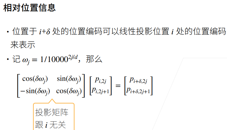
        # 编码公式:X[i, j] = sin(i / 10000^(2j / num_hiddens)) 或 cos(i / 10000^(2j / num_hiddens))
        X = torch.arange(max_len, dtype=torch.float32).reshape(
            -1, 1) / torch.pow(10000,
                               torch.arange(0, num_hiddens, 2, dtype=torch.float32) /
                               num_hiddens)
        # 将位置编码矩阵中的偶数维度的元素替换为sin函数的结果
        self.P[:,:,0::2] = torch.sin(X)
        # 将位置编码矩阵中的奇数维度的元素替换为cos函数的结果
        self.P[:,:,1::2] = torch.cos(X)

    # 前向传播函数,接收输入张量X作为输入
    def forward(self, X):
        # 将位置编码张量P与输入张量X相加,并将结果移动到与X相同的设备上
        X = X + self.P[:, :X.shape[1], :].to(X.device)
        # 对相加后的结果应用dropout,并返回结果
        return self.dropout(X)
python
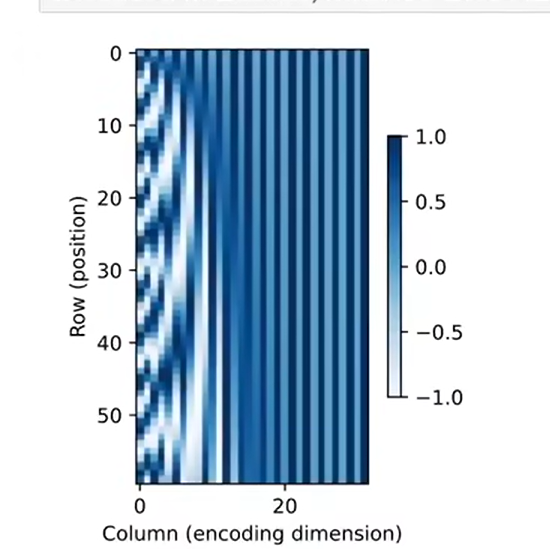
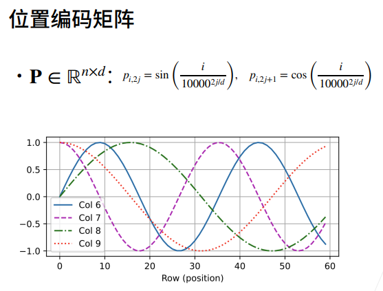
# 行代表标记在序列中的位置,列代表位置编码的不同维度
# 设置位置编码的维度和序列的长度
encoding_dim, num_steps = 32, 60
# 创建位置编码器实例,传入位置编码的维度和dropout率
pos_encoding = PositionalEncoding(encoding_dim, 0)
# 将位置编码器设置为评估模式,不进行训练
pos_encoding.eval()
# 应用位置编码器到全0张量上,得到位置编码后的张量X
X = pos_encoding(torch.zeros((1, num_steps, encoding_dim)))
# 获取位置编码器中的位置编码张量P,截取与X相同长度的部分
P = pos_encoding.P[:, :X.shape[1], :]
# 绘制位置编码张量P中特定维度的子集
d2l.plot(torch.arange(num_steps), P[0, :, 6:10].T, xlabel='Row (position)',
figsize=(6, 2.5), legend=["Col %d" % d for d in torch.arange(6, 10)]) 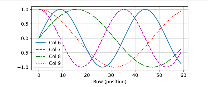
python
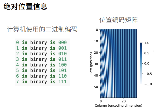
# 循环遍历范围为0到7的数字
for i in range(8):
    # 打印当前数字的二进制表示,使用字符串格式化进行对齐和补零
print(f'{i} in binary is {i:>03b}')0 in binary is 000
1 in binary is 001
2 in binary is 010
3 in binary is 011
4 in binary is 100
5 in binary is 101
6 in binary is 110
7 in binary is 111
python
# 在编码维度上降低频率
# 从位置编码张量P中获取第一个样本的编码部分,并添加两个维度
P = P[0, :, :].unsqueeze(0).unsqueeze(0)
# 显示热力图,以编码维度为x轴,位置为y轴
d2l.show_heatmaps(P, xlabel='Column (encoding dimension)',
                 ylabel='Row (position)', figsize=(3.5, 4), cmap='Blues')