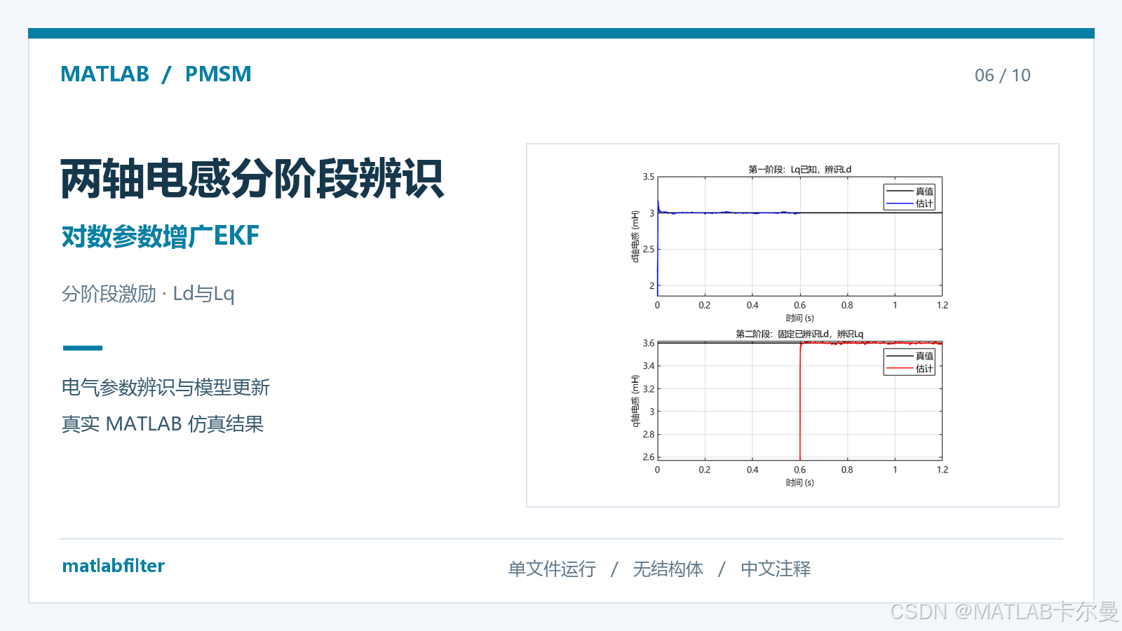
'程序有中文注释,可直接运行、得到结果`
文章目录
程序简介
本程序基于MATLAB搭建永磁同步电机(Permanent Magnet Synchronous Motor,PMSM)电气仿真模型,采用增广扩展卡尔曼滤波(Extended Kalman Filter,EKF),实现d轴电感和q轴电感的分阶段辨识,并对参数估计精度及滤波性能进行分析。
在永磁同步电机运行过程中,d轴和q轴电感是影响电流动态响应、电磁转矩计算及控制系统性能的重要参数。准确辨识两轴电感,有助于提高电机数学模型的准确性,为后续参数补偿和控制算法研究提供参考。
算法原理与实现
程序采用对数参数增广EKF,将待辨识的电感参数与dq轴电流共同纳入状态向量,利用已知转速、dq轴电压及带噪电流量测,完成状态预测、协方差传播和滤波更新。
与同时估计两个电感参数的方法不同,本例采用分阶段辨识策略:
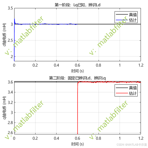
- 第一阶段:d轴电感辨识。 在q轴电感已知的条件下,通过增广EKF估计d轴电感Ld。
- 第二阶段:q轴电感辨识。 将第一阶段末段得到的Ld估计均值作为已知参数,重新初始化滤波器,对q轴电感Lq进行辨识。
程序使用对数参数形式保证辨识结果为正,并采用Joseph形式更新误差协方差,同时通过数值差分核对模型雅可比矩阵。
仿真场景与结果分析
程序构建了具有理想编码器转速信息的电气仿真环境,通过多频电流指令产生不同的dq轴电压与电流响应,为电感参数辨识提供激励条件。
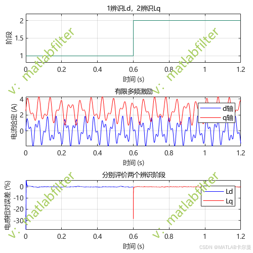
仿真总时长为1.2秒,其中前0.6秒用于d轴电感辨识,后0.6秒用于q轴电感辨识。两轴电感真实值保持恒定,主要考察算法的参数收敛能力和估计误差。
程序主要输出以下结果:
- 两轴电感辨识曲线: 分别展示Ld和Lq的真实值与估计值,观察参数收敛过程。
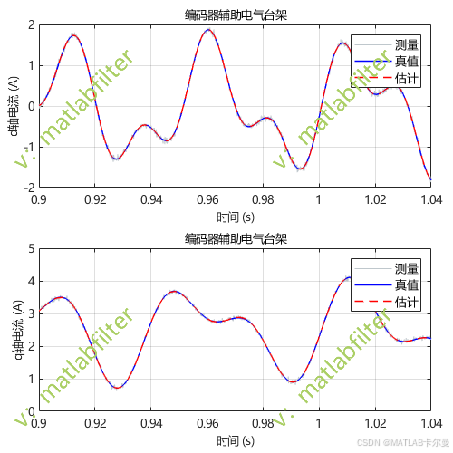
- dq轴电流滤波结果: 对比真实电流、带噪测量电流和滤波估计电流。
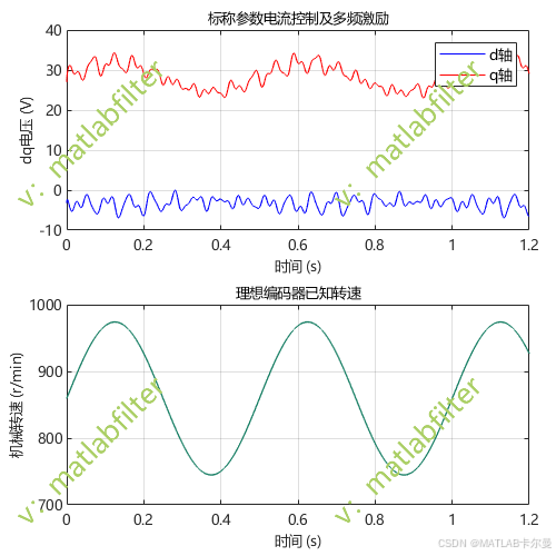
- 电压激励与转速变化: 展示电机运行过程中施加的dq轴电压及已知机械转速。
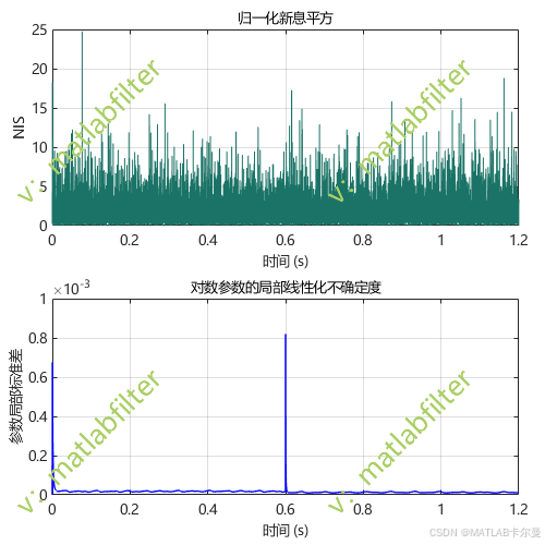
- 新息与参数不确定度: 展示归一化新息平方(NIS)和参数估计标准差,辅助分析滤波过程。
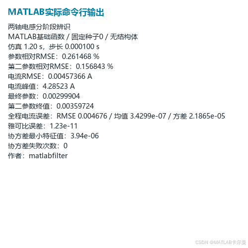
- 分阶段辨识误差: 展示不同辨识阶段的电感相对误差,并输出均方根误差(RMSE)等评价指标。
程序特点与适用方向
本程序使用基础MATLAB函数实现,包含完整的电机电气模型、参数初始化、分阶段EKF辨识、数值计算检查以及结果可视化过程。
电机电阻、d-q轴电感、永磁磁链、采样时间、电流激励、测量噪声及滤波协方差等参数均可自行调整,方便开展不同参数配置下的仿真测试。
本例适用于永磁同步电机参数辨识、扩展卡尔曼滤波、电机电气模型分析及在线参数估计等方向的学习与研究,也可作为进一步研究多参数联合辨识和电机参数补偿方法的参考。
运行结果
dq电流滤波
两轴电感辨识
分阶段激励与电感误差
新息与参数不确定度
电压激励与编码器转速
命令行输出
MATLAB源代码
部分代码如下:
matlab
% 两轴电感分阶段辨识:独立MATLAB例程
% 2026-10-09/Ver1,作者:matlabfilter,V同号,可获取代码定制、讲解等
% 只使用基础MATLAB。参数为普通标量,信号为数值数组,不使用结构体。
% 点击运行即可;末尾含全部局部函数。Figure无水印,配套PNG由维护工具导出。
clear; clc; close all;
rng(0);

%% 共用教学参数与单位:不将本例解释为Word中15 kW电机的实机验证
Rs=0.45; Ld=3e-3; Lq=3.6e-3; psi_f=0.075;
pole_pairs=4; J=2e-3; B=5e-4;
Ts=1e-4; simulation_time=1.2;
dc_voltage=120; voltage_limit=dc_voltage/sqrt(3); current_limit=10;
Kp_speed=0.25; Ki_speed=4.0;
current_bandwidth=1200;
Kp_d=Ld*current_bandwidth; Kp_q=Lq*current_bandwidth;
Ki_d=Rs*current_bandwidth; Ki_q=Rs*current_bandwidth;
time=0:Ts:simulation_time; sample_count=numel(time);
Kt=1.5*pole_pairs*psi_f; Kr=1.5*pole_pairs*(Ld-Lq);
% 维护用汇总也是数值向量;各指标仍以独立、有意义的变量保留。
speed_rmse=NaN; angle_rmse_deg=NaN; load_rmse=NaN;
parameter_relative_rmse_pct=NaN; secondary_parameter_rmse_pct=NaN;
improvement_pct=NaN; current_rmse=NaN; peak_speed_error=NaN;
gap_speed_rmse=NaN; recovery_speed_rmse=NaN;
final_parameter=NaN; final_secondary_parameter=NaN;
disturbance_speed_peak=NaN; control_current_peak=NaN; takeover_speed_peak=NaN;
recovery_time=NaN; covariance_min=Inf; covariance_chol_failures=0;
jacobian_error=0; state_is_finite=1;

%% 理想有编码器电气台架:机械转速已知,只研究电气参数
speed_known=90+12*sin(2*pi*2*time);
angle_known=cumtrapz(time,pole_pairs*speed_known);
id_reference=1.2*sin(2*pi*19*time)+0.7*sin(2*pi*43*time);
iq_reference=2.5+1.1*sin(2*pi*17*time)+0.7*sin(2*pi*31*time);
resistance_true=Rs*ones(1,sample_count);
flux_true=psi_f*ones(1,sample_count);
Ld_true=Ld*ones(1,sample_count); Lq_true=Lq*ones(1,sample_count);

current_true=zeros(2,sample_count); current_true(:,1)=[0;2.5];
voltage_dq=zeros(2,sample_count); current_integrals=zeros(2,1);
for k=2:sample_count
    [udq,current_integrals]=dq_current_controller(current_true(:,k-1), ...
        [id_reference(k-1);iq_reference(k-1)],speed_known(k-1),current_integrals,Ts, ...
        Rs,Ld,Lq,psi_f,pole_pairs,Kp_d,Ki_d,Kp_q,Ki_q,voltage_limit);
    voltage_dq(:,k-1)=udq;
    current_true(:,k)=electrical_truth_step(current_true(:,k-1),udq,speed_known(k-1), ...
        Ts,resistance_true(k-1),Ld_true(k-1),Lq_true(k-1),flux_true(k-1),pole_pairs);
end
voltage_dq(:,end)=voltage_dq(:,end-1);
current_dq_meas=current_true+0.04*randn(2,sample_count);

%% 对数参数增广EKF:不输入待辨识参数真值
x=[current_dq_meas(:,1);log(0.75)]; P=diag([0.2^2,0.2^2,0.3^2]);
Q=diag([2e-6,2e-6,2e-7]); R=0.04^2*eye(2); H=[eye(2),zeros(2,1)];
state_est=zeros(3,sample_count); state_est(:,1)=x;
innovation=nan(2,sample_count); nis_values=nan(1,sample_count);
parameter_sigma=zeros(1,sample_count);
Ld_known=Ld; Lq_known=Lq;
axis_index=1; parameter_nominal=Ld; switch_index=find(time>=0.60,1);
Ld_est=nan(1,sample_count); Lq_est=nan(1,sample_count); Ld_est(1)=Ld*exp(x(3));
phase_index=ones(1,sample_count); phase_index(switch_index:end)=2;
jacobian_error=max(check_electrical_jacobian(Rs,Ld,Lq,psi_f,pole_pairs,Ts,1),check_electrical_jacobian(Rs,Ld,Lq,psi_f,pole_pairs,Ts,2));
assert(jacobian_error<1e-6,'电气模型离散雅可比核对失败');
for k=2:sample_count
    if k==switch_index
        % 第二阶段使用第一阶段尾段均值,不读取Ld真值。
        Ld_known=mean(Ld_est(time>=0.50 & time<0.60));
        axis_index=2; parameter_nominal=Lq;
        x=[current_dq_meas(:,k-1);log(0.75)]; P=diag([0.2^2,0.2^2,0.3^2]);
    end
    [xp,F]=electrical_predict(x,voltage_dq(:,k-1),speed_known(k-1),Ts, ...
        Rs,Ld_known,Lq_known,psi_f,pole_pairs,axis_index);
    Pp=F*P*F'+Q;
    residual=current_dq_meas(:,k)-H*xp;
    S=H*Pp*H'+R; K=(Pp*H')/S;

    x=xp+K*residual;
    IKH=eye(3)-K*H; P=IKH*Pp*IKH'+K*R*K'; P=(P+P')/2;
    state_est(:,k)=x; innovation(:,k)=residual; nis_values(k)=residual'*(S\residual);
    parameter_value=parameter_nominal*exp(x(3));
    parameter_sigma(k)=parameter_value*sqrt(P(3,3));
    if axis_index==1, Ld_est(k)=parameter_value; else, Lq_est(k)=parameter_value; end
    [~,chol_flag]=chol(P); covariance_chol_failures=covariance_chol_failures+(chol_flag~=0);
    covariance_min=min(covariance_min,min(eig(P)));
    assert(chol_flag==0 && all(isfinite(x)) && parameter_value>0,'参数或协方差异常');
end
current_est=state_est(1:2,:);
current_error=current_est-current_true;
current_rmse=sqrt(mean(current_error(:,time>=0.24).^2,'all'));
control_current_peak=max(abs(current_true),[],'all');
first_evaluation=time>=0.40 & time<0.60; second_evaluation=time>=1.00;
parameter_relative_rmse_pct=100*sqrt(mean(((Ld_est(first_evaluation)-Ld)./Ld).^2));
secondary_parameter_rmse_pct=100*sqrt(mean(((Lq_est(second_evaluation)-Lq)./Lq).^2));
final_parameter=Ld_known; final_secondary_parameter=Lq_est(end);

%% 绘图:Figure保持无水印,不在商品代码中写入图片
make_figure('两轴电感辨识'); tiledlayout(2,1,'TileSpacing','compact','Padding','compact');
nexttile; plot(time,Ld_true*1e3,'k-',time,Ld_est*1e3,'b-','LineWidth',1.1);
decorate_axes('时间 (s)','d轴电感 (mH)','第一阶段:Lq已知,辨识Ld'); legend('真值','估计');
nexttile; plot(time,Lq_true*1e3,'k-',time,Lq_est*1e3,'r-','LineWidth',1.1);
decorate_axes('时间 (s)','q轴电感 (mH)','第二阶段:固定已辨识Ld,辨识Lq'); legend('真值','估计');
make_figure('dq电流滤波'); tiledlayout(2,1,'TileSpacing','compact','Padding','compact');
for axis=1:2
    nexttile; plot(time,current_dq_meas(axis,:),'Color',[0.75 0.78 0.8]); hold on;
    plot(time,current_true(axis,:),'b-',time,current_est(axis,:),'r--','LineWidth',1);
    if axis==1, label='d轴电流 (A)'; else, label='q轴电流 (A)'; end
    decorate_axes('时间 (s)',label,'编码器辅助电气台架'); xlim([0.90 1.04]); legend('测量','真值','估计');
end
make_figure('电压激励与编码器转速'); tiledlayout(2,1,'TileSpacing','compact','Padding','compact');
nexttile; plot(time,voltage_dq(1,:),'b-',time,voltage_dq(2,:),'r-','LineWidth',0.8);
decorate_axes('时间 (s)','dq电压 (V)','标称参数电流控制及多频激励'); legend('d轴','q轴');
nexttile; plot(time,speed_known*30/pi,'Color',[0.1 0.5 0.4],'LineWidth',1);
decorate_axes('时间 (s)','机械转速 (r/min)','理想编码器已知转速');
make_figure('新息与参数不确定度'); tiledlayout(2,1,'TileSpacing','compact','Padding','compact');
nexttile; plot(time,nis_values,'Color',[0.1 0.45 0.4]);
decorate_axes('时间 (s)','NIS','归一化新息平方');
nexttile; plot(time,parameter_sigma,'b-','LineWidth',1);
decorate_axes('时间 (s)','参数局部标准差','对数参数的局部线性化不确定度');
make_figure('分阶段激励与电感误差'); tiledlayout(3,1,'TileSpacing','compact','Padding','compact');
nexttile; stairs(time,phase_index,'Color',[0.1 0.5 0.4]);
decorate_axes('时间 (s)','阶段','1辨识Ld,2辨识Lq'); ylim([0.8 2.2]);
nexttile; plot(time,id_reference,'b-',time,iq_reference,'r-');
decorate_axes('时间 (s)','电流给定 (A)','有限多频激励'); legend('d轴','q轴');
nexttile; plot(time,100*(Ld_est-Ld)/Ld,'b-',time,100*(Lq_est-Lq)/Lq,'r-');
decorate_axes('时间 (s)','电感相对误差 (%)','分别评价两个辨识阶段'); legend('Ld','Lq');

%% 命令行统计与独立数值输出
完整代码:
如需帮助,或有滤波相关的MATLAB代码定制需求,可从个人主页左侧联系我