一、问题描述
近期围绕imu总是出现问题,自己整理了一下将数据可视化的工具
二、imu 类
1. 待处理数据格式
bash
#  yaw     roll        pitch     time
-2.08131 -0.0741765 0.0200713 121.281000000
-2.08724 -0.0745256 0.0197222 121.301000000
-2.093 -0.0757473 0.018326 121.321000000
-2.09789 -0.0774926 0.0164061 121.341000000
-2.10138 -0.0792379 0.0144862 121.361000000
-2.10452 -0.0808087 0.0122173 121.381000000
-2.10836 -0.082205 0.0102974 121.401000000
-2.11377 -0.0834267 0.00820305 121.421000000
-2.1204 -0.0842994 0.00663225 121.441000000
-2.1286 -0.084823 0.00523599 121.461000000
-2.13873 -0.0849975 0.00418879 121.481000000
2. matlab 源程序
matlab
clc;
% 0: 选择对话框 1:文件路径(默认)
mode=1;
% 选择打开文件方式
switch mode
% 选择对话框打开文件
case 0
[filename, pathname] = uigetfile('*.txt', 'Select the IMU data log file');
if isequal(filename, 0)
disp('User selected Cancel');
return;
else
disp(['User selected ', fullfile(pathname, filename)]);
end
% 打开文件路径获取文件
case 1
% file_name="all_roate";
file_name="sensor_data_2";
pathname="/home/work/IMU/imu_rviz/imu_data/";
file=file_name+".txt";
otherwise
disp("Other Case ...");
end
% 完整的文件路径
filepath = fullfile(pathname, file);
data = importdata(filepath);
%************************************* 计算当前角度 ***********************************************
% 提取yaw, roll, pitch和时间
y_yaw = data(:, 1); % 第1列是yaw
y_roll = data(:, 2); % 第2列是roll
y_pitch = data(:, 3); % 第3列是pitch
x_time = data(:, 4); % 第4列是时间
% 创建折线图
figure;
markerSize = 2; % 设置数据点的尺寸
plot(x_time, y_yaw, '-o', 'Color', 'b','MarkerSize', markerSize, 'DisplayName', 'Yaw'); % 绘制Yaw数据
hold on; % 保持当前图表
plot(x_time, y_roll, '-o', 'Color', 'r', 'MarkerSize', markerSize, 'DisplayName', 'Roll'); % 绘制Roll数据
plot(x_time, y_pitch, '-o', 'Color', 'g','MarkerSize', markerSize, 'DisplayName', 'Pitch'); % 绘制Pitch数据
% 设置图表标题和标签
title([file_name, ' - Angle Display'], 'Interpreter', 'none');
xlabel('Time (s)');
ylabel('IMU Angle (rad)');
h_legend = legend('show'); % 显示图例
grid on; % 启用网格线
grid minor; % 启用次要网格线
% 设置图表充满figure
set(gca, 'Position', [0.035, 0.05, 0.95, 0.9]); % 使Axes充满figure窗口(left, bottom, width, height)
% 设置图例项的可点击属性
h_legend.ItemHitFcn = @toggleVisibility;
%************************************* 计算前后帧角度差 ***********************************************
% 计算角度差并进行归一化
yaw_diff = diff(y_yaw);
yaw_diff = mod(yaw_diff + pi, 2*pi) - pi; % 将角度差限制在 -π 到 π 之间
yaw_diff = [yaw_diff; 0]; % 最后一帧差值设为0
roll_diff = diff(y_roll);
roll_diff = mod(roll_diff + pi, 2*pi) - pi; % 将角度差限制在 -π 到 π 之间
roll_diff = [roll_diff; 0]; % 最后一帧差值设为0
pitch_diff = diff(y_pitch);
pitch_diff = mod(pitch_diff + pi, 2*pi) - pi; % 将角度差限制在 -π 到 π 之间
pitch_diff = [pitch_diff; 0]; % 最后一帧差值设为0
% 创建新的图窗并绘制角度差折线图
figure;
% plot(x_time, yaw_diff, '-*', 'Color', 'b', 'DisplayName', 'Yaw Difference'); % 绘制Yaw差值
% hold on;
% plot(x_time, roll_diff, '-x', 'Color', 'r', 'DisplayName', 'Roll Difference'); % 绘制Roll差值
% plot(x_time, pitch_diff, '-x', 'Color', 'g', 'DisplayName', 'Pitch Difference'); % 绘制Pitch差值
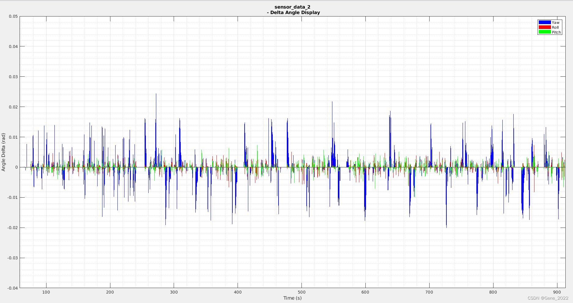
bar(x_time, yaw_diff, 'FaceColor', 'b', 'DisplayName', 'Yaw'); % 绘制Yaw差值
hold on;
bar(x_time, roll_diff, 'FaceColor', 'r', 'DisplayName', 'Roll'); % 绘制Roll差值
bar(x_time, pitch_diff, 'FaceColor', 'g', 'DisplayName', 'Pitch'); % 绘制Pitch差值
% 设置图表标题和标签
title([file_name, ' - Delta Angle Display'], 'Interpreter', 'none');
xlabel('Time (s)');
ylabel('Angle Delta (rad)');
D_legend = legend('show'); % 显示图例
grid on; % 启用网格线
grid minor; % 启用次要网格线
% 设置图表充满figure
set(gca, 'Position', [0.035, 0.05, 0.95, 0.9]); % 使Axes充满figure窗口(left, bottom, width, height)
D_legend.ItemHitFcn = @toggleVisibility;
%************************************* 计算前后帧时间差 ***********************************************
% 计算时间戳差值
time_diff = diff(x_time); % 计算相邻时间戳之间的差值
time_diff = [time_diff; 0]; % 最后一个时间戳差值设为0,因为没有下一帧
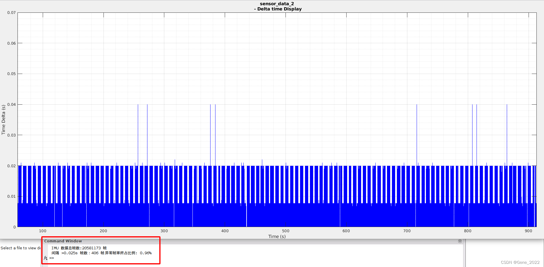
% 统计 time_diff > 0.025 的次数及其比例
threshold = 0.025;
data_sum=sum(data(:));
count_exceed = sum(time_diff > threshold); % 计算超过阈值的数量
total_count = length(time_diff); % 总的时间戳差值数量
proportion_exceed = count_exceed / total_count; % 计算超过阈值的比例
% 打印统计结果
fprintf(' IMU 数据总帧数:%.f 帧 \n', data_sum);% 打印数据总和,不采用科学计数法
fprintf(' 间隔 >%.3fs 帧数:%d 帧\t', threshold, count_exceed);
fprintf('异常帧率所占比例: %.2f%%\n', proportion_exceed * 100);
% 创建新的图窗并绘制柱状图
figure;
bar(x_time, time_diff, 'FaceColor', 'b'); % 绘制时间戳差值柱状图
% 设置图表标题和标签
title([file_name, ' - Delta time Display'], 'Interpreter', 'none');
xlabel('Time (s)');
ylabel('Time Delta (s)');
grid on; % 启用网格线
grid minor; % 启用次要网格线
% 设置图表充满figure
set(gca, 'Position', [0.035, 0.05, 0.95, 0.9]); % 使Axes充满figure窗口(left, bottom, width, height)
%************************************* 函数置于程序最后 ***********************************************
% 回调函数,用于显示和隐藏折线
function toggleVisibility(~, event)
h_line = event.Peer;
% 切换折线的可见性
if strcmp(h_line.Visible, 'on')
h_line.Visible = 'off';
else
h_line.Visible = 'on';
end
end三、效果
注意 :点击图例,图表中对应折线可显示与隐藏。

三、RTK类
1. 待处理数据格式
bash
# 	p_x						p_y 						p_z						lat						lon 			alt		type sats	time
0.932831314024 0.688128449856 -0.065349213413 31.189889848090 120.593791473480 12.1707 50 23 264.971752582
0.933988519921 0.686419487272 -0.067954306696 31.189889832690 120.593791485610 12.1681 50 23 265.062251207
0.934132574159 0.686145386414 -0.066855122953 31.189889830220 120.593791487120 12.1692 50 23 265.174277166
0.930754446656 0.689859606514 -0.069844054392 31.189889863690 120.593791451710 12.1662 50 23 265.262168874
0.930238330538 0.691429854924 -0.070039372782 31.189889877840 120.593791446300 12.1660 50 23 265.371954541
0.926209575172 0.691106926309 -0.076640334879 31.189889874930 120.593791404070 12.1594 50 23 265.462255416
0.926119897413 0.692730441288 -0.074935496950 31.189889889560 120.593791403130 12.1611 50 23 265.571762541
0.925914784963 0.693109963431 -0.077834364811 31.189889892980 120.593791400980 12.1582 50 23 265.662138374
2. matlab 源程序
matlab
clc;
% 0: 选择对话框 1:文件路径(默认)
mode=1;
% 选择打开文件方式
switch mode
% 选择对话框打开文件
case 0
[filename, pathname] = uigetfile('*.txt', 'Select the IMU data log file');
if isequal(filename, 0)
disp('User selected Cancel');
return;
else
disp(['User selected ', fullfile(pathname, filename)]);
end
% 打开文件路径获取文件
case 1
% file_name="all_roate";
file_name="rtk_data";
pathname="/home/work/IMU/imu_rviz/imu_data/";
file=file_name+".txt";
otherwise
disp("Other Case ...");
end
% 完整的文件路径
filepath = fullfile(pathname, file);
data = importdata(filepath);
% %************************************* 数据提取 ***********************************************
% 提取yaw, roll, pitch和时间
p_x = data(:, 1); % 第1列是x
p_y = data(:, 2); % 第2列是y
p_z = data(:, 3); % 第3列是z
p_time = data(:, 9); % 第9列是时间
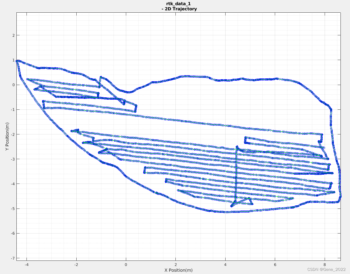
%************************************ 二维图绘制 *********************************************
figure;
markerSize = 4; % 设置数据点的尺寸
plot(p_x, p_y, '-o','MarkerSize', markerSize, 'LineWidth', 0.1, 'Color', 'b');
title([file_name, ' - 2D Trajectory'], 'Interpreter', 'none');
xlabel('X Position(m)');
ylabel('Y Position(m)');
hold on;
grid on;
grid minor; % 启用次要网格线
axis equal;
set(gca, 'Position', [0.035, 0.05, 0.9, 0.9]); % 使Axes充满figure窗口(left, bottom, width, height)
% 计算箭头的方向向量
u = diff(p_x);
v = diff(p_y);
% 在所有点上绘制箭头
quiver(p_x(1:end-1), p_y(1:end-1), u, v, 0, 'MaxHeadSize', 0.2, 'Color', 'g');
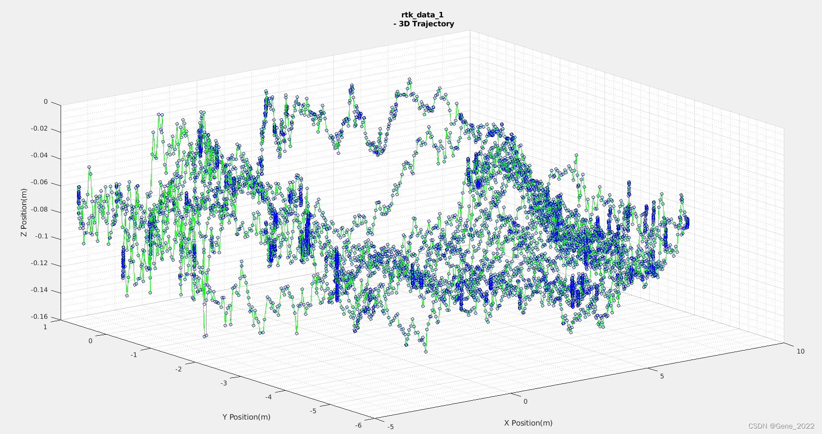
%************************************ 三维图绘制 *********************************************
figure;
plot3(p_x, p_y, p_z, '-o','MarkerSize', markerSize, 'LineWidth', 0.1, 'Color', 'b');
title([file_name, ' - 3D Trajectory'], 'Interpreter', 'none');
xlabel('X Position(m)');
ylabel('Y Position(m)');
zlabel('Z Position(m)');
grid on;
grid minor; % 启用次要网格线
view(3); % 设置默认的三维视角
hold on;
% 计算三维箭头的方向向量
u3 = diff(p_x);
v3 = diff(p_y);
w3 = diff(p_z);
% 在所有点上绘制三维箭头
quiver3(p_x(1:end-1), p_y(1:end-1), p_z(1:end-1), u3, v3, w3, 0, 'MaxHeadSize', 0.2, 'Color', 'g');
hold off;
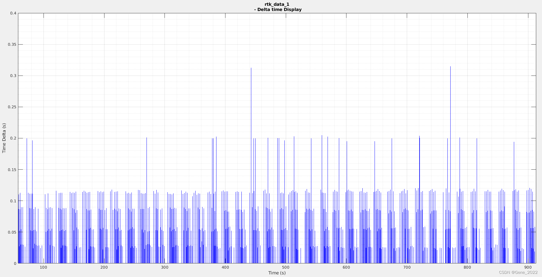
%************************************* 计算前后帧时间差 ***********************************************
% 计算时间戳差值
time_diff = diff(p_time); % 计算相邻时间戳之间的差值
time_diff = [time_diff; 0]; % 最后一个时间戳差值设为0,因为没有下一帧
% 统计 time_diff > 0.025 的次数及其比例
threshold = 0.15;
data_sum=sum(data(:));
count_exceed = sum(time_diff > threshold); % 计算超过阈值的数量
total_count = length(time_diff); % 总的时间戳差值数量
proportion_exceed = count_exceed / total_count; % 计算超过阈值的比例
% 打印统计结果
fprintf(' RTK 数据总帧数:%.f 帧 \n', data_sum);% 打印数据总和,不采用科学计数法
fprintf(' 间隔 >%.3fs 帧数:%d 帧\t', threshold, count_exceed);
fprintf('异常帧率所占比例: %.2f%%\n', proportion_exceed * 100);
% 创建新的图窗并绘制柱状图
figure;
bar(p_time, time_diff, 'FaceColor', 'b'); % 绘制时间戳差值柱状图
% 设置图表标题和标签
title([file_name, ' - Delta time Display'], 'Interpreter', 'none');
xlabel('Time (s)');
ylabel('Time Delta (s)');
grid on; % 启用网格线
grid minor; % 启用次要网格线
% 设置图表充满figure
set(gca, 'Position', [0.035, 0.05, 0.95, 0.9]); % 使Axes充满figure窗口(left, bottom, width, height)
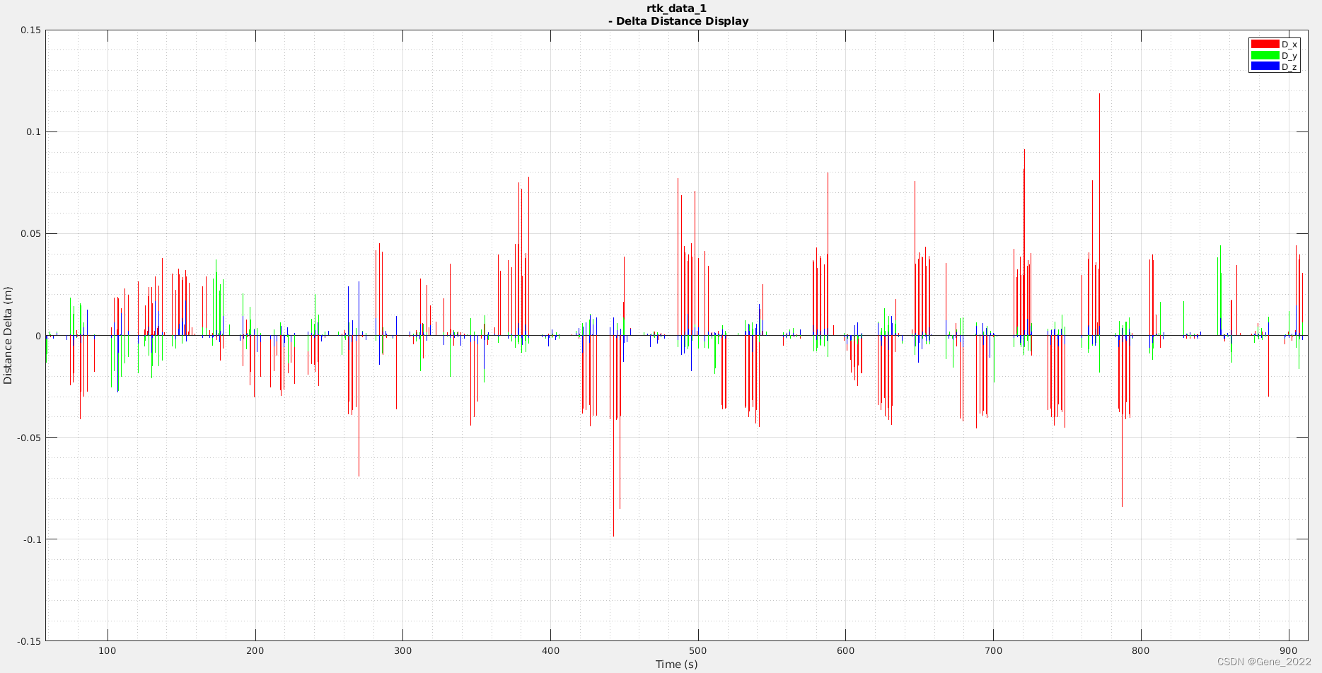
%************************************* 计算前后帧距离差 ***********************************************
% 计算角度差并进行归一化
x_diff = diff(p_x);
x_diff = [x_diff; 0]; % 最后一帧差值设为0
y_diff = diff(p_y);
y_diff = [y_diff; 0]; % 最后一帧差值设为0
z_diff = diff(p_z);
z_diff = [z_diff; 0]; % 最后一帧差值设为0
% 创建新的图窗并绘制角度差折线图
figure;
bar(p_time, x_diff, 'FaceColor', 'r', 'DisplayName', 'D\_x'); % 绘制Yaw差值
hold on;
bar(p_time, y_diff, 'FaceColor', 'g', 'DisplayName', 'D\_y'); % 绘制Roll差值
bar(p_time, z_diff, 'FaceColor', 'b', 'DisplayName', 'D\_z'); % 绘制Pitch差值
% 设置图表标题和标签
title([file_name, ' - Delta Distance Display'], 'Interpreter', 'none');
xlabel('Time (s)');
ylabel('Distance Delta (m)');
D_legend = legend('show'); % 显示图例
grid on; % 启用网格线
grid minor; % 启用次要网格线
% 设置图表充满figure
set(gca, 'Position', [0.035, 0.05, 0.95, 0.9]); % 使Axes充满figure窗口(left, bottom, width, height)
D_legend.ItemHitFcn = @toggleVisibility;
%************************************* 函数置于程序最后 ***********************************************
% 回调函数,用于显示和隐藏折线
function toggleVisibility(~, event)
h_line = event.Peer;
% 切换折线的可见性
if strcmp(h_line.Visible, 'on')
h_line.Visible = 'off';
else
h_line.Visible = 'on';
end
end三、效果
注意 :点击图例,图表中对应折线可显示与隐藏,二维、三维缩放图表箭头由当前帧指向下一帧。