一、背景介绍
2007 年的全球经济危机深刻改变了世界经济格局,引发了一系列连锁反应,波及各大洲。经济增长停滞不前,甚至在某些情况下出现负增长,给出口导向型发展中国家带来了不确定性。实体经济受到的冲击尤为严重,生产成本上升,利润下降,实际经济价值缩水。相比之下,金融部门的投资活动激增,原因是在动荡的经济环境中寻求稳定和更高的回报。然而,金融投资的性质与实体经济有很大不同,实体经济的特点是复杂且往往不可预测的因素交织在一起。。。。。
二、研究现状
理解和掌握标准普尔 500 指数的变化规律,对于正确评估美国经济趋势、跟踪世界经济发展的源和流、参与全球市场套利和定价具有重要的现实意义。基于标准普尔 500 指数在金融市场中的重要地位,标准普尔 500 指数的预测受到研究人员的更多关注。
目前对标准普尔 500 指数的研究主要集中在短期预测上,使用不同的研究工具。例如,1在预测标准普尔 500 指数值时使用隐马尔可夫链方法和离散时间马尔可夫链方法,指出使用全样本数据和特征子样本时预测效果更好。。。。。。
三、数据集介绍和分析
3.1 数据分析
在这项研究中,选择了美国股票的标准普尔 500 指数进行预测分析,并初步选择开盘价、最高价、最低价和收盘价作为研究数据。
标准普尔 500 指数的数据收集时间为 1995 年 1 月 3 日至 2020 年 12 月 31 日,包括该期间内的交易日。
R
library(quantmod)
library(TTR)

data$Date <- as.Date(data$Date, format = "%Y/%m/%d")

# (VWAP)
data$VWAP <- with(data, rowSums(data[, c("High", "Low", "Close")]) / 3 * Volume / sum(data$Volume))
R
#### Convert data to xts objects
HTM_xts <- xts(HTM[, c("Open", "High", "Low", "Close")], order.by = HTM$Date)


plot(HTM_xts)
addLegend("topleft", legend.names = colnames(HTM_xts), lwd = 1)
3.2稳定性分析
该检验的原假设和备择假设为:
原假设:该序列存在单位根。
备择假设:该序列不存在单位根。
如果我们不能拒绝原假设,我们可以说该序列是非平稳的。

以收盘价为例,通过上图我们可以看出,该指数的均值和标准差都在增加,初步判断该序列是非平稳的。
表 1. 单位根检验的结果
|--------------------|----------|---------------|---------|
| | Variable | ADF Statistic | p value |
| Dickey-Fuller Test | Open | -0.428 | 0.985 |
| Dickey-Fuller Test | High | -0.250 | 0.990 |
| Dickey-Fuller Test | Low | -0.525 | 0.981 |
| Dickey-Fuller Test | Close | -0.442 | 0.984 |
从表 1 中,我们观察到所有四个时间序列的 p 值都大于 0.05。因此,我们不能拒绝原假设,并得出时间序列是非平稳的结论。为了解决这个问题,我们需要对序列进行差分。

|--------------------|----------|---------------|---------|
| | Variable | ADF Statistic | p value |
| Dickey-Fuller Test | Open | -18.943 | 0.010 |
| Dickey-Fuller Test | High | -18.834 | 0.010 |
| Dickey-Fuller Test | Low | -18.697 | 0.010 |
| Dickey-Fuller Test | Close | -18.742 | 0.010 |
四、方法理论
向量自回归(VAR)模型是自回归(AR)模型的扩展,是一种常用的计量经济模型6。它考虑了多个变量之间的相互依赖关系,比简单的 AR 模型更全面。。。。。
五、模型建立和分析
选择 1995-01-03 至 2020-11-16 期间作为训练集,预测 2020-11-17 至 2020-12-31 期间的数据。
|----|--------|--------|--------|--------------|
| | AIC(n) | HQ(n) | SC(n) | FPE(n) |
| 1 | 17.678 | 17.686 | 17.699 | 47606900.000 |
| 2 | 17.073 | 17.086 | 17.111 | 25986330.000 |
| 3 | 16.810 | 16.829 | 16.865 | 19983500.000 |
| 4 | 16.735 | 16.759 | 16.805 | 18523240.000 |
| 5 | 16.583 | 16.613 | 16.670 | 15910690.000 |
| 6 | 16.513 | 16.549 | 16.617 | 14837310.000 |
| 7 | 16.442 | 16.484 | 16.563 | 13826240.000 |
| 8 | 16.391 | 16.439 | 16.529 | 13139830.000 |
| 9 | 16.307 | 16.360 | 16.461 | 12075260.000 |
| 10 | 16.273 | 16.332 | 16.444 | 11673230.000 |
我们可以看到,不同的标准选择了相同的滞后长度(n=10)。当滞后长度超过 3 时,AIC 值的下降幅度变小,这表明在 3 之后添加更多的滞后观测值并不会显著提高模型拟合度。因此,按照选择 AIC 值较小的更简单模型的原则,我们选择 p=3 作为滞后阶数。
|----------|----------|-----------|---------|-----------------|
| Estimation results for equation Open: |||||
| Open = Open.l1 + High.l1 + Low.l1 + Close.l1 + Open.l2 + High.l2 + Low.l2 + Close.l2 + Open.l3 + High.l3 + Low.l3 + Close.l3 + const |||||
| | Estimate | Std.Error | t value | Pr(>|t|) |
| Open.l1 | -0.840 | 0.018 | -45.764 | < 2e-16 *** |
| High.l1 | -0.004 | 0.016 | -0.229 | 0.819 |
| Low.l1 | 0.043 | 0.014 | 3.079 | 0.00209 ** |
| Close.l1 | 0.897 | 0.012 | 72.094 | < 2e-16 *** |
| Open.l2 | -0.309 | 0.020 | -15.594 | < 2e-16 *** |
| High.l2 | -0.113 | 0.019 | -6.031 | 1.72e-09 *** |
| Low.l2 | 0.001 | 0.016 | 0.072 | 0.943 |
| Close.l2 | 0.820 | 0.018 | 44.881 | < 2e-16 *** |
| Open.l3 | -0.011 | 0.013 | -0.852 | 0.395 |
| High.l3 | -0.108 | 0.016 | -6.676 | 2.66e-11 *** |
| Low.l3 | -0.017 | 0.014 | -1.200 | 0.230 |
| Close.l3 | 0.367 | 0.016 | 22.711 | < 2e-16 *** |
| const | 0.135 | 0.093 | 1.449 | 0.147 |
| Signif. codes: 0 '***' 0.001 '**' 0.01 '*' 0.05 '.' 0.1 ' ' 1 |||||
| Residual standard error: 7.522 on 6499 degrees of freedom |||||
| Multiple R-Squared: 0.8063, Adjusted R-squared: 0.8059 |||||
| F-statistic: 2254 on 12 and 6499 DF, p-value: < 2.2e-16 |||||
|----------|----------|-----------|---------|-----------------|
| Estimation results for equation High: |||||
| High = Open.l1 + High.l1 + Low.l1 + Close.l1 + Open.l2 + High.l2 + Low.l2 + Close.l2 + Open.l3 + High.l3 + Low.l3 + Close.l3 + const |||||
| | Estimate | Std.Error | t value | Pr(>|t|) |
| Open.l1 | -0.196 | 0.030 | -6.592 | 4.69e-11 *** |
| High.l1 | -0.680 | 0.026 | -25.885 | < 2e-16 *** |
| Low.l1 | 0.041 | 0.023 | 1.815 | 0.06952 . |
| Close.l1 | 0.698 | 0.020 | 34.741 | < 2e-16 *** |
| Open.l2 | 0.133 | 0.032 | 4.164 | 3.16e-05 *** |
| High.l2 | -0.538 | 0.030 | -17.707 | < 2e-16 *** |
| Low.l2 | -0.018 | 0.026 | -0.714 | 0.475 |
| Close.l2 | 0.715 | 0.030 | 24.222 | < 2e-16 *** |
| Open.l3 | 0.111 | 0.021 | 5.308 | 1.14e-07 *** |
| High.l3 | -0.324 | 0.026 | -12.385 | < 2e-16 *** |
| Low.l3 | -0.015 | 0.022 | -0.658 | 0.511 |
| Close.l3 | 0.281 | 0.026 | 10.743 | < 2e-16 *** |
| const | 0.391 | 0.151 | 2.592 | 0.00955 ** |
| Signif. codes: 0 '***' 0.001 '**' 0.01 '*' 0.05 '.' 0.1 ' ' 1 |||||
| Residual standard error: 12.15 on 6499 degrees of freedom |||||
| Multiple R-Squared: 0.3167, Adjusted R-squared: 0.3154 |||||
| F-statistic: 251 on 12 and 6499 DF, p-value: < 2.2e-16 |||||
模型检验
为了确保模型已经捕获了数据中的所有方差和模式,我们需要测试残差项中是否存在剩余相关性。
|---------------------|--------|--------------------|
| Portmanteau Test (asymptotic) |||
| Chi-squared = 850.9 | df = 0 | p-value < 2.2e-16 |
非常小的 p 值表明拒绝了无自相关的原假设。这是一个信号,表明需要增加滞后长度。我们可以考虑在 VAR 模型中选择更高的滞后阶数,以使残差中的自相关在很大程度上被消除。以"Close"为例,可以看出模型的预测性能不是很令人满意(见图 5)。

R
comparison_df <- data.frame(
  date = forecast_df$date,
  forecasted = forecast_df$close,
  actual = test_o$Close
)
comparison_df

ggplot(comparison_df, aes(x = date)) +
  geom_line(aes(y = forecasted, color = "Forecasted")) +
  geom_line(aes(y = Close, color = "Actual")) +
  labs(x = "Date", y = "Close Value", color = "Data") +
  scale_color_manual(values = c("Forecasted" = "blue", "Actual" = "red")) +
  theme_minimal()+
  theme(panel.border = element_rect(color = "black", fill = NA),
        panel.grid.major = element_blank(),
        panel.grid.minor = element_blank())
四个指数的预测误差在 50 左右。
|------|--------|--------|--------|--------|
| | Open | High | Low | Close |
| RMSE | 54.559 | 54.141 | 57.482 | 58.794 |
可视化结果如下
R
###plot
rmse_open <- 54.55896
rmse_high <- 54.14115
rmse_low <- 57.48235
rmse_close <- 58.79398


rmse_data <- data.frame(
  RMSE = c(rmse_open, rmse_high, rmse_low, rmse_close),
  Type = c("Open", "High", "Low", "Close")
)


barplot(rmse_data$RMSE,
        names.arg = rmse_data$Type,
        main = "RMSE Values",
        xlab = "Type",
        ylab = "RMSE",
        col = rainbow(length(rmse_data$RMSE)))


text(x = 1:length(rmse_data$RMSE),
     y = rmse_data$RMSE,
     label = round(rmse_data$RMSE, 2),
     pos = 3,
     cex = 0.8,
     col = "black",
xpd = TRUE) 
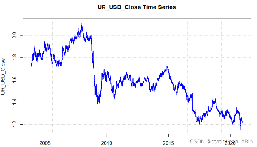
接下来,使用欧美汇率数据对 S&P 500 股票价格和其他特征进行多元线性回归:
|-------------|----------|------------|---------|------------------|
| Call: |||||
| lm(formula = dataset$UR_USD Close ~ log_Open + log_High + log_Low + log_Close, data = dataset) |||||
| Residuals: |||||
| Min | 1Q | Median | 3Q | Max |
| -0.48796 | -0.09936 | -0.02465 | 0.08142 | 0.48518 |
| Coefficients: |||||
| | Estimate | Std. Error | t value | Pr(>|t|) |
| (Intercept) | 4.80613 | 0.05312 | 90.480 | < 0.0000 *** |
| log_Open | 0.51837 | 0.61270 | 0.846 | 0.397575 |
| log_High | -2.27459 | 0.66081 | -3.442 | 0.0006 *** |
| log_Low | 1.98556 | 0.56573 | 3.510 | 0.000453 *** |
| log_Close | -0.65925 | 0.59302 | -1.112 | 0.266336 |
| Signif. codes: 0 '***' 0.001 '**' 0.01 '*' 0.05 '.' 0.1 ' ' 1 |||||
| Residual standard error: 0.1658 on 4297 degrees of freedom Multiple R-squared: 0.4693, Adjusted R-squared: 0.4689 F-statistic: 950.1 on 4 and 4297 DF, p-value: < 0.00000000000000022 |||||
从上述模型拟合结果可以看出,去除对数后的每日最高价和每日最低价是最显著的水平,因此从理论上讲,它们对欧美汇率有影响。
六、结论
在这项研究中,VAR 模型被用于对标准普尔 500 指数的开盘价、最高价、最低价和收盘价进行多变量预测。然而,我们的分析表明,虽然 VAR 模型在捕捉一些变量之间的线性关系方面表现良好,但它可能无法完全捕捉非线性驱动因素的影响。随后,我们使用欧美汇率数据,结合标准普尔 500 股票和其他特征的数据,对数据进行多元线性回归和对数处理,最终结果表明,标准普尔 500 指数的每日最高价和最低价对欧元兑美元汇率有显著影响。
在未来的实验过程中,可以选择特征进行进一步的影响分析,如脉冲响应和方差分解等,这些可以继续探索影响因素,同时为经济投资提供一定程度的指导。
七、参考文献
1Hashemi, Ray R., et al. Extraction of the Essential Constituents of the S&P 500 Index. 2017 international conference on computational science and computational intelligence (CSCI). IEEE, 2017.
2Sukparungsee, S. . A comparison of s&p 500 index forecasting models of arima, arima with garch-m and arima with e-garch.International Journal of Technical Research and Applications,32,2015.
3K.J.M. Cremers. Stock return predictability. a Bayesian model selection perspective. Rev. Financ. Stud,15(4), 1223--1249,2002.
4Wang F .Predicting S&P 500 Market Price by Deep Neural Network and Enemble ModelJ.E3S Web of Conferences, 2020.DOI:10.1051/e3sconf/202021402040.
5G. M. Siddesh,et al.A Long Short-Term Memory Network-Based Approach for Predicting the Trends in the S&P 500 Index.Journal of The Institution of Engineers.1(105),19-26,2024.
创作不易,希望大家多多点赞收藏和评论!