文章目录
- [项目三 关联规则分析](#项目三 关联规则分析)
注意 任务二:痹症方剂用药规律分析
项目三 关联规则分析
一、实践目的
- 了解关联规则算法原理;
- 熟悉关联规则应用场景;
- 掌握使用 Apriori算法、FP-grouth算法进行关联规则分析的方法;
二、实践平台
- 操作系统:Windows7及以上
- Python版本:3.8.x及以上
- PyCharm或 Anoconda集成环境
三、实践内容
任务一:在线购物车分析
针对数据集 Online Retail.xlsx进行预处理。该数据集记录了在 2010年 12月 01日至 2011年 12月 09日的 541909条在线交易记录,包含 8个属性,主要属性如下:
- InvoiceNo: 订单编号,由 6位整数表示,退货单号由字母"C"开头。
- StockCode: 产品编号,每个不同的产品由不重复的 5位整数表示。
- Description: 产品描述。
- Quantity: 产品数量,每笔交易的每件产品的数量。
- InvoiceDate: 订单日期和时间,表示生成每笔交易的日期和时间。
- UnitPrice: 单价,单位产品的英镑价格。
- CustomerID: 顾客编号,每个客户由唯一的 5位整数表示。
- Country: 国家名称,每个客户所在国家/地区的名称。
(一)数据读入
- 导入本案例所需的 Python包;
- 将数据读入并存为 DataFrame格式,查看前 5行数据。
(二)数据理解
- 调用 shape属性查看数据集的形状;
- 调用 describe()方法对数据集进行探索性分析;
- 调用 info()方法查看样本数据的相关信息概览;
- 查看国家列(country)的取值;
- 查看各国家的购物数量;
- 查看订单编号(invoiceno)一列中是否有重复值;
(三)数据预处理
- 查看数据集中是否有缺失值;
- 删除商品名称(description)一列的字符串头尾的空白字符;
- 查看商品名称(description)一列的缺失值个数,并去除缺失值;
- 由于退货的订单编号由字母"C"开头,删除含有 C字母的已取消订单,并查看数据集形状;
- 将数据改为每一行一条购物记录(只计算德国客户),并查看结果的前 5行;
- 由于 Apriori方法中 df参数允许的值为 0/1或 True/False,在此将上面处理后的数据集转换为 0/1的形式;
(四)生成频繁项集
- mlxtend.frequent_patterns的 apriori()方法可以进行频繁项集的计算,将最小支持度设定为 0.07;输出结果,并查看满足条件的频繁项集个数;
- 使用 fpgrowth()方法寻找频繁项集,最小支持度设为 0.05;输出结果,查看满足条件的频繁项集个数;
(五)计算关联度
- 将提升度(lift)作为度量计算关联规则,并设置阈值为 1,表示计算具有正相关关系的关联规则,请通过 mlxtend.frequent_patterns的 association_rules()方法实现,并输出计算结果;
- 在以上结果中筛选出提升度不小于 2且置信度不小于 0.8的关联规则,并输出结果;
(六)可视化
通过 matplotlib.pyplot的 scatter函数绘制出提升度不小于1的关联规则的散点图,横坐标设置为支持度,纵坐标为置信度,散点的大小表示提升度。
(七)Apriori参数及其解读
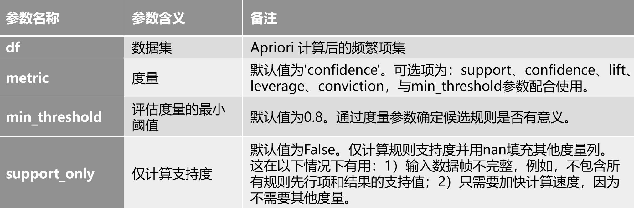
(八)association_rules参数及其解读

任务二:用药规律分析
数据集"痹症方剂.xls"记录了治疗痹症的用药药方,请使用关联规则算法生成频繁项集,并计算关联度。(最小支持度及支持度、提升度等度量指标可自行决定。)
四、结果提交
提交任务一和任务二的全部实现代码。
任务一:在线购物车分析
python
import pandas as pd
from mlxtend.frequent_patterns import apriori, fpgrowth
from mlxtend.frequent_patterns import association_rules
import warnings

# 忽略所有的 DeprecationWarning
warnings.filterwarnings("ignore", category=DeprecationWarning)

# (一)数据读入
# 1. 导入本案例所需的 Python 包;
# 2. 将数据读入并存为 DataFrame 格式,查看前 5 行数据。
data = pd.read_excel('input/Online Retail.xlsx')
print(data.head(5))
python
# (二)数据理解

# 1. 调用 shape 属性查看数据集的形状;
print(data.shape)
# 2. 调用 describe()方法对数据集进行探索性分析;
print(data.describe())
# 3. 调用 info()方法查看样本数据的相关信息概览;
print(data.info())
# 4. 查看国家列(country)的取值;
print(data['Country'].unique())
# 5. 查看各国家的购物数量;
print(data['Country'].value_counts())
# 6. 查看订单编号(invoiceno)一列中是否有重复值;
print('重复值的数量', data['InvoiceNo'].duplicated().sum())
python
(541909, 8)
            Quantity                    InvoiceDate      UnitPrice  \
count  541909.000000                         541909  541909.000000
mean        9.552250  2011-07-04 13:34:57.156386048       4.611114
min    -80995.000000            2010-12-01 08:26:00  -11062.060000
25%         1.000000            2011-03-28 11:34:00       1.250000
50%         3.000000            2011-07-19 17:17:00       2.080000
75%        10.000000            2011-10-19 11:27:00       4.130000
max     80995.000000            2011-12-09 12:50:00   38970.000000
std       218.081158                            NaN      96.759853

          CustomerID
count  406829.000000
mean    15287.690570
min     12346.000000
25%     13953.000000
50%     15152.000000
75%     16791.000000
max     18287.000000
std      1713.600303
<class 'pandas.core.frame.DataFrame'>
RangeIndex: 541909 entries, 0 to 541908
Data columns (total 8 columns):
 #   Column       Non-Null Count   Dtype
---  ------       --------------   -----
 0   InvoiceNo    541909 non-null  object
 1   StockCode    541909 non-null  object
 2   Description  540455 non-null  object
 3   Quantity     541909 non-null  int64
 4   InvoiceDate  541909 non-null  datetime64[ns]
 5   UnitPrice    541909 non-null  float64
 6   CustomerID   406829 non-null  float64
 7   Country      541909 non-null  object
dtypes: datetime64[ns](1), float64(2), int64(1), object(4)
memory usage: 33.1+ MB
None
['United Kingdom' 'France' 'Australia' 'Netherlands' 'Germany' 'Norway'
 'EIRE' 'Switzerland' 'Spain' 'Poland' 'Portugal' 'Italy' 'Belgium'
 'Lithuania' 'Japan' 'Iceland' 'Channel Islands' 'Denmark' 'Cyprus'
 'Sweden' 'Austria' 'Israel' 'Finland' 'Bahrain' 'Greece' 'Hong Kong'
 'Singapore' 'Lebanon' 'United Arab Emirates' 'Saudi Arabia'
 'Czech Republic' 'Canada' 'Unspecified' 'Brazil' 'USA'
 'European Community' 'Malta' 'RSA']
Country
United Kingdom          495478
Germany                   9495
France                    8557
EIRE                      8196
Spain                     2533
Netherlands               2371
Belgium                   2069
(三)数据预处理
python
# 1. 查看数据集中是否有缺失值;
print(data.isnull().sum())
# 2. 删除商品名称(description)一列的字符串头尾的空白字符;
data['Description'] = data['Description'].str.strip()
# 3. 查看商品名称(description)一列的缺失值个数,并去除缺失值;
print(data['Description'].isnull().sum())
data = data.dropna(subset=['Description'])
python
InvoiceNo           0
StockCode           0
Description      1454
Quantity            0
InvoiceDate         0
UnitPrice           0
CustomerID     135080
Country             0
dtype: int64
1455
python
# 4. 由于退货的订单编号由字母"C"开头,删除含有 C 字母的已取消订单,并查看数据集形状;
data = data[~data['InvoiceNo'].astype(str).str.startswith('C')]
print(data.shape)
# 5. 将数据改为每一行一条购物记录(只计算德国客户),并查看结果的前 5 行;
data_germany = data[data['Country'] == 'Germany']
data_germany = data_germany.groupby(['InvoiceNo', 'Description'])['Quantity'].sum().unstack().reset_index().fillna(
    0).set_index('InvoiceNo')
data_germany = data_germany.map(lambda x: 1 if x > 0 else 0)
print(data_germany.head())
(四)生成频繁项集
python
# 1. 使用 apriori() 方法进行频繁项集的计算,将最小支持度设定为 0.07;输出结果,并查看满足条件的频繁项集个数;
frequent_itemsets_apriori = apriori(data_germany,
                                    min_support=0.07,
                                    use_colnames=True)
# 输出频繁项集结果
print("频繁项集(Apriori 方法):")
print(frequent_itemsets_apriori)

# 输出满足条件的频繁项集个数
print("满足条件的频繁项集个数:", len(frequent_itemsets_apriori))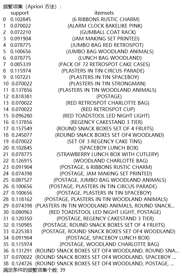
python
# 2. 使用 fpgrowth()方法寻找频繁项集,最小支持度设为 0.05;输出结果,查看满足条件的频繁项集个数;
frequent_itemsets_fpgrowth = fpgrowth(data_germany,
                                      min_support=0.05,
                                      use_colnames=True)

# 输出频繁项集结果
print("频繁项集(FP-Growth 方法):")
print(frequent_itemsets_fpgrowth)

# 输出满足条件的频繁项集个数
print("满足条件的频繁项集个数:", len(frequent_itemsets_fpgrowth))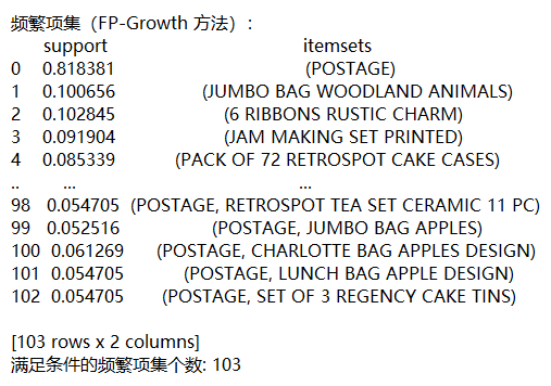
(五)计算关联度
python
# 1. 将提升度(lift)作为度量计算关联规则,并设置阈值为 1,表示计算具有正相关关系的关联规则,请通过 association_rules() 方法实现,并输出计算结果;
# 计算提升度并生成关联规则
rules = association_rules(frequent_itemsets_apriori,
                          metric="lift",
                          min_threshold=1)

# 输出关联规则结果
print("生成的关联规则:")
print(rules)
python
# 2. 在以上结果中筛选出提升度不小于 2 且置信度不小于 0.8 的关联规则,并输出结果;
filtered_rules = rules[(rules['lift'] >= 2) & (rules['confidence'] >= 0.8)]

# 输出筛选结果
print("筛选后的关联规则:")
print(filtered_rules)
# 保存输出结果
filtered_rules.to_csv('output/filtered_rules.csv')
可视化结果
python
# 通过 matplotlib.pyplot的 scatter 函数绘制出提升度不小于1的关联规则的散点图,横坐标设置为支持度,纵坐标为置信度,散点的大小表示提升度。

import matplotlib.pyplot as plt

# 正常显示
plt.rcParams['font.sans-serif'] = ['SimHei']  # 用来正常显示中文标签
# 显示符号
plt.rcParams['axes.unicode_minus'] = False  # 用来正常显示负号
# 筛选提升度不小于 1 的关联规则
filtered_rules = rules[rules['lift'] >= 1]

# 绘制散点图
plt.figure(figsize=(10, 6))
scatter = plt.scatter(filtered_rules['support'], filtered_rules['confidence'],
                      s=filtered_rules['lift'] * 100,  # 散点大小,放大提升度便于观察
                      alpha=0.5,  # 散点透明度
                      c='blue',  # 散点颜色
                      edgecolors='w')  # 散点边缘颜色

# 添加标签和标题
plt.title('关联规则的散点图(支持度 vs 置信度)')
plt.xlabel('支持度')
plt.ylabel('置信度')

# 添加每个点的标注(可选)
# for i in range(filtered_rules.shape[0]):
#     plt.annotate(filtered_rules.index[i],
#                  (filtered_rules['support'].iloc[i],
#                   filtered_rules['confidence'].iloc[i]),
#                  fontsize=8)

plt.grid()
plt.show()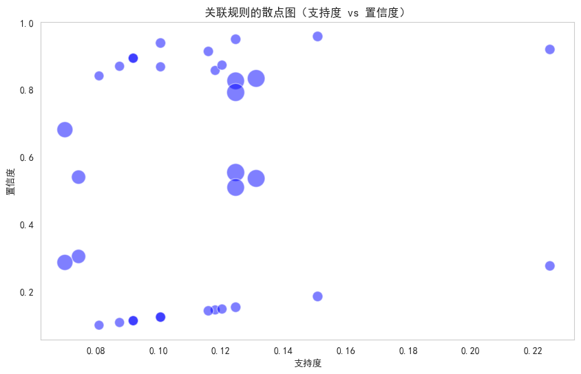
任务二:用药规律分析
python
import pandas as pd
from mlxtend.frequent_patterns import apriori, association_rules
from mlxtend.preprocessing import TransactionEncoder


# 1. 读取数据
data = pd.read_excel("input/痹症方剂.xls")
print(data)

print("\n数据的基本信息:")
print(data.info())
python
# 2. 数据预处理
# 转换DataFrame为事务格式
def encode_items(x):
    return [item for item in x if str(item) != 'nan']

transactions = data.apply(encode_items, axis=1)

# 创建事务编码器对象并拟合数据
te = TransactionEncoder()
te_ary = te.fit(transactions).transform(transactions)
df_te = pd.DataFrame(te_ary, columns=te.columns_)

# 应用Apriori算法找到频繁项集
frequent_itemsets = apriori(df_te, min_support=0.05, use_colnames=True)
print(frequent_itemsets)
python
      support        itemsets
0    0.977528              ()
1    0.067416            (丹参)
2    0.067416            (乳香)
3    0.191011            (人参)
4    0.067416            (僵蚕)
..        ...             ...
151  0.056180  (, 桂心, 甘草, 人参)
152  0.056180  (, 茯苓, 甘草, 人参)
153  0.056180  (, 防风, 甘草, 人参)
154  0.056180  (, 当归, 甘草, 防风)
155  0.056180  (, 茯苓, 桂心, 甘草)
python
# 计算关联规则
rules = association_rules(frequent_itemsets, metric="lift", min_threshold=1)
print(rules)

# 保存频繁项集和关联规则
frequent_itemsets.to_csv('output/test2_frequent_itemsets.csv')
rules.to_csv('output/test2_rules.csv')

python
# 通过 matplotlib.pyplot的 scatter 函数绘制出提升度不小于1的关联规则的散点图,横坐标设置为支持度,纵坐标为置信度,散点的大小表示提升度。

import matplotlib.pyplot as plt

# 正常显示
plt.rcParams['font.sans-serif'] = ['SimHei']  # 用来正常显示中文标签
# 显示符号
plt.rcParams['axes.unicode_minus'] = False  # 用来正常显示负号
# 筛选提升度不小于 1 的关联规则
filtered_rules = rules[rules['lift'] >= 1]

# 绘制散点图
plt.figure(figsize=(10, 6))
scatter = plt.scatter(filtered_rules['support'], filtered_rules['confidence'],
                      s=filtered_rules['lift'] * 100,  # 散点大小,放大提升度便于观察
                      alpha=0.5,  # 散点透明度
                      c='blue',  # 散点颜色
                      edgecolors='w')  # 散点边缘颜色

# 添加标签和标题
plt.title('关联规则的散点图(支持度 vs 置信度)')
plt.xlabel('支持度')
plt.ylabel('置信度')

# 添加每个点的标注(可选)
# for i in range(filtered_rules.shape[0]):
#     plt.annotate(filtered_rules.index[i],
#                  (filtered_rules['support'].iloc[i],
#                   filtered_rules['confidence'].iloc[i]),
#                  fontsize=8)

plt.grid()
plt.show()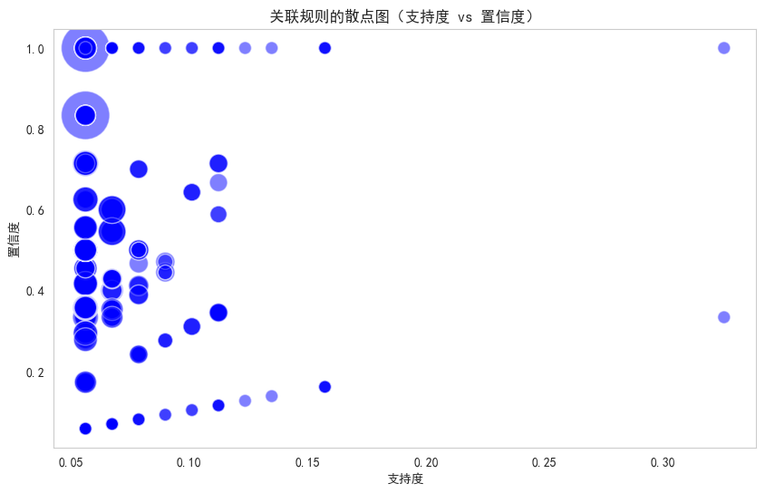
任务二的运行结果,我并不满意,但是没有找到优化方法。若有良策,望指点一二。