文章目录
- 1.引用
- 2.内置图片数据集加载
- 3.处理为batch类型
- 4.设置运行设备
- 5.查看数据
- 6.绘图查看数据图片
- 7.定义卷积函数
- 8.卷积实例化、损失函数、优化器
- 9.训练和测试损失、正确率
- 10.额外添加
1.引用
torchvision提供了一些常用的数据集、模型、转换函数等
python
import torchvision
from torchvision import transforms
import numpy as np
import matplotlib.pyplot as plt
2.内置图片数据集加载
torch的内置图片数据集均在datasets模块下,包含Catletch、CelebA、CIFAR、Cityscapes、COCO、Fashion-MNIST、ImageNet、MNIST等。
MNIST数据集是0-9手写数字数据集。
train=True表示是训练数据
torchvision.transforms包含了转换函数
这里用到了ToTensor类,该类的主要作用有以下3点:
①将输入转换成张量
②读取图片的格式规范为(channel,heigth,width)
③将图片像素的取值范围归一化0-1
python
train_ds=torchvision.datasets.MNIST('data/',train=True,transform=transforms.ToTensor(),download=True)
test_ds=torchvision.datasets.MNIST('data/',train=False,transform=transforms.ToTensor(),download=True)
3.处理为batch类型
DataLoader有以下4个目的:
①使用shuffle参数对数据集做乱序的操作(随机打乱)
②将数据采样为小批次,可用batch_size参数指定批次大小(小批次)
③可以充分利用多个子进程加速数据预处理(多线程)
④可通过collate_fn参数传递批次数据中的处理函数,实现对批次数据进行转换处理(转换处理)
python
train_dl=torch.utils.data.DataLoader(train_ds,batch_size=64,shuffle=True)
test_dl=torch.utils.data.DataLoader(test_ds,batch_size=64) 上述两行代码创建了DataLoader类型的train_dl和test_dl
DataLoader是可迭代对象,next方法返回一个批次的图像imgs和对应一个批次的标签labels
4.设置运行设备
机器学习或者深度学习需要选择程序运行的设备是CPU还是GPU,GPU就是通常所说的需要有显卡。
python
device='cuda' if torch.cuda.is_available() else 'cpu'
print('use {} device'.format(device))
5.查看数据
python
imgs,labels=next(iter(train_dl))
print(imgs.shape)
print(labels.shape)
结果:
torch.Size([64, 1, 28, 28])
torch.Size([64])
6.绘图查看数据图片
imgs[:10]查看前10条数据
np.squeeze从数组的形状中删除维度为 1 的维度。
np.unsqueeze从数组的形状中添加维度为 1 的维度。
注:只有数组长度在该维度上为 1,那么该维度才可以被删除。如果不是1,那么删除的话会报错
报错信息:cannot select an axis to squeeze out which has size not equal to one
(1)不显示图片标签
python
plt.figure(figsize=(10,1))
for i,img in enumerate(imgs[:10]):
    npimg=img.numpy()
    npimg=np.squeeze(npimg)#形状由(1,28,28)转换为(28,28)
    plt.subplot(1,10,i+1)
    plt.imshow(npimg)      #在子图中绘制单张图片
    plt.axis('off')        #关闭显示子图坐标
print(labels[:10])
plt.show()
(2)打印图片标签
python
classes = ('0', '1', '2', '3', '4', '5', '6', '7', '8', '9')
class_label_str=''

img_label_list=list(zip(imgs,labels))
for i,(img,label) in enumerate(img_label_list):
    nimg=np.array(img)
    nimg=np.squeeze(nimg)
    plt.subplot(8,8,i+1)
    plt.title(str(label.item()))
    plt.imshow(nimg)
    plt.axis('off')
    '''按照图片显示格式打印所有标签:i!=0实现按行打印的同时第一行前面无空行,按每行8列打印'''
    if i!=0 and i%8==0:
        class_label_str +='\n'
    class_label_str += classes[label.item()]+'\t'
print(class_label_str)
plt.show()
(3)图片显示标签
我这里以'airplane', 'automobile', 'bird', 'cat', 'deer', 'dog', 'frog', 'horse', 'ship', 'truck'这些类别示例,作用于手写字体图像分类时,要更改成0-9
python
classes = ('airplane', 'automobile', 'bird', 'cat', 'deer', 'dog', 'frog', 'horse', 'ship', 'truck')

img_label_list=list(zip(imgs,labels))
for i,(img,label) in enumerate(img_label_list):
    nimg=img.transpose(0, 2)
    nimg=nimg.numpy()
    plt.subplot(5,5,i+1)
    plt.title(classes[label.item()])
    plt.imshow(nimg)
    plt.axis('off')
plt.show()
7.定义卷积函数
定义卷积函数才是算法模型的真正开始,卷积层一般是必不可少的,是机器学习和深度学习的灵魂与基石所在。
python
class net(nn.Module):
    def __init__(self):
        super().__init__()
        self.conv1=nn.Conv2d(1,6,5)
        self.conv2=nn.Conv2d(6,16,5)
        self.linear1 = nn.Linear(16*4*4,20)
        self.linear2 = nn.Linear(20,10)

    def forward(self,input):
        x=torch.max_pool2d(torch.relu(self.conv1(input)),2)
        x=torch.max_pool2d(torch.relu(self.conv2(x)),2)
        x=x.view(x.size(0),-1)
        x=torch.relu(self.linear1(x))
        x=self.linear2(x)
        return x
算法模型流程示意:

8.卷积实例化、损失函数、优化器
python
model=net().to(device)
loss_f=nn.CrossEntropyLoss()
opti=optim.Adam(model.parameters(), lr=0.005)
9.训练和测试损失、正确率
(1)训练
python
def train(dataloader,model,loss_f,opt):
    model.train()                  #模型为训练模式
    num_batches=len(dataloader)    #总批次数
    size=len(dataloader.dataset)   #样本总数(所有的批次里所有的数据点)
    loss_zhi=0                     #所有批次的损失之和
    correct=0                      #预测正确的样本总数

    for x,y in dataloader:
        x,y=x.to(device),y.to(device)
        pred=model(x)
        loss=loss_f(pred,y)
        '''梯度清零、反向传播、梯度更新是专属'''
        opt.zero_grad()
        loss.backward()
        opt.step()

        with torch.no_grad():
        loss_zhi+=loss.item()
            correct+=(pred.argmax(1)==y).type(torch.float).sum().item()

    loss_zhi/=num_batches  #loss_zhi是所有批次的损失之和,所以计算全部样本的平均损失需要除以总批次数
    correct/=size          #correct是预测正确的样本总数,若计算每个批次总体正确率,需除以样本总数量
return loss_zhi,correct 注:当前代码里的pred.argmax(1)会返会类似Tensor([4,6,...,0])的Tensor,而y也是类似形状的tensor,因此二者可以用==比较
(2)测试
python
def test(dataloader, model):
    model.eval()                   #模型为测试模式
    num_batches=len(dataloader)    #总批次数
    size=len(dataloader.dataset)   #样本总数(所有的批次里所有的数据点)
    loss_zhi=0                     #所有批次的损失之和
    correct=0                      #预测正确的样本总数

    for x, y in dataloader:
        x,y=x.to(device),y.to(device)
        pred = model(x)
        loss = loss_f(pred, y)

        with torch.no_grad():
        loss_zhi += loss.item()
            correct += (pred.argmax(1) == y).type(torch.float).sum().item()
    loss_zhi /= num_batches
    correct /= size
    return loss_zhi, correct
(3)循环
python
epochs = 200
train_loss = []
train_acc = []
test_loss = []
test_acc = []
for epoch in range(epochs):
    epoch_train_loss,epoch_train_acc=train(train_dl,model,loss_f,opt)
    epoch_test_loss,epoch_test_acc=test(test_dl,model)

    train_loss.append(epoch_train_loss)
    train_acc.append(epoch_train_acc)
    test_loss.append(epoch_test_loss)
    test_acc.append(epoch_test_acc)

    tishi='epoch:{},train_loss:{:.4f},train_acc:{:.2f}%,test_loss:{:.4f},test_acc:{:.2f}%'
    print(tishi.format(epoch,train_loss[-1],train_acc[-1]*100,test_loss[-1],test_acc[-1]*100))
print('batch over!')
(4)损失和正确率曲线
python
plt.figure(figsize=(10,4))
plt.subplot(121)
#打印损失
plt.plot(range(1,epochs+1),train_loss,label='train_loss')
plt.plot(range(1,epochs+1),test_loss,label='test_loss')
plt.title('train+test:loss')
plt.xlabel('epoch')
plt.legend(loc='upper right')
plt.subplot(122)
#打印正确率
plt.plot(range(1,epochs+1),train_acc,label='train_acc')
plt.plot(range(1,epochs+1),test_acc,label='test_acc')
plt.title('train+test:acc')
plt.xlabel('epoch')
plt.legend(loc='lower right')
plt.show()
plt.savefig('D:/loss+acc.png')
(5)输出数据到表格
python
table={'train_loss':train_loss,
        'train_acc':train_acc,
        'test_loss':test_loss,
        'test_acc':test_acc}
data_shuju=pd.DataFrame(table,index=list(range(1,epochs+1)))
data_shuju.to_excel('D:/loss+acc.xlsx')
10.额外添加
(1)添加dropout减少过拟合
卷积后添加Dropout层较少使用,效果也不是很明显,这是因为相邻元素之间有相关性,随机地丢弃卷积输出特征像素点,抑制过拟合的效果有限。
Dropout的第一个参数是输入的tensor,第二个参数p代表的是丢弃的神经元的比例,默认为0.5。
①未添加dropout层
python
class net(nn.Module):
    def __init__(self):
        super().__init__()
        self.conv1=nn.Conv2d(1,6,5)
        self.conv2=nn.Conv2d(6,16,5)
        self.linear1 = nn.Linear(16*4*4,20)
        self.linear2 = nn.Linear(20,10)

    def forward(self,input):
        x=torch.max_pool2d(torch.relu(self.conv1(input)),2)
        x=torch.max_pool2d(torch.relu(self.conv2(x)),2)
        x=x.view(x.size(0),-1)
        x=torch.relu(self.linear1(x))
        x=self.linear2(x)
return x dropout前loss+acc图像:

②添加dropout层
python
class net(nn.Module):
    def __init__(self):
        super().__init__()
        self.conv1=nn.Conv2d(1,6,5)
        self.conv2=nn.Conv2d(6,16,5)
        self.linear1 = nn.Linear(16*4*4,20)
        self.linear2 = nn.Linear(20,10)

    def forward(self,input):
        x=torch.max_pool2d(torch.relu(self.conv1(input)),2)
        x=torch.max_pool2d(torch.relu(self.conv2(x)),2)
        x=x.view(x.size(0),-1)
        x=torch.dropout(x, p=0.5, train=self.training)
        x=torch.relu(self.linear1(x))
        x=torch.dropout(x, p=0.5, train=self.training)
        x=self.linear2(x)
return x dropout后loss+acc图像:

(2)循环同时输出时间
python
import time

epochs=1
train_loss=[]
train_acc=[]
test_loss=[]
test_acc=[]
epoch_time=[]
start=time.time()
for epoch in range(epochs):
    epoch_train_loss,epoch_train_acc=train(train_dl,model,loss_f,opt)
    epoch_test_loss, epoch_test_acc = test(test_dl, model)

    train_loss.append(epoch_train_loss)
    train_acc.append(epoch_train_acc)
    test_loss.append(epoch_test_loss)
    test_acc.append(epoch_test_acc)
    epoch_time.append(time.time()-start)
    tishi='epoch:{},train_loss:{:.4f},train_acc:{:.2f}%,test_loss:{:.4f},test_acc:{:.2f}%,time:{:.2f}'
    print(tishi.format(epoch,train_loss[-1],train_acc[-1]*100,test_loss[-1],test_acc[-1]*100,epoch_time[-1]))
print('epoch over!')

table={'train_loss':train_loss,
        'train_acc':train_acc,
        'test_loss':test_loss,
        'test_acc':test_acc,
        'epoch_time':epoch_time}
data_shuju=pd.DataFrame(table,index=list(range(1,epochs+1)))
data_shuju.to_excel('loss+acc.xlsx')
print('save over!')
(3)每个类别分类正确率输出
①输出到控制台
注:需要在网络循环loss+acc之后使用,若是提前使用正确率只有个位数
python
class_correct = list(0 for i in range(10))  #每个类别预测正确的数量
class_total   = list(0 for i in range(10))  #每个类别的总数量
with torch.no_grad():
    # 从测试数据中取出数据
    for x, y in test_dl:
        x, y= x.to(device), y.to(device)
        outputs = model(x)
        _, predicted = torch.max(outputs, 1)
        # 预测正确的返回True,预测错误的返回False;squeeze将数据转换为一维数据
        c = (predicted == y).squeeze()
        for i in range(10):
            label = y[i]  # 提取标签
            class_correct[label] += c[i].item()  # 预测正确个数
            class_total[label] += 1  # 总数
for i in range(10):
    print('{}的准确率:{:.2f}%'.format(classes[i], 100 * class_correct[i] / class_total[i]))
结果:
0的准确率:98.03%
1的准确率:100.00%
2的准确率:100.00%
3的准确率:98.08%
4的准确率:97.74%
5的准确率:97.62%
6的准确率:98.44%
7的准确率:99.39%
8的准确率:98.60%
9的准确率:97.60%
②输出到表格
python
class_test_dic={}
for i in range(10):
    print('{:.10s}的准确率:{:.2f}%'.format(classes[i], 100 * class_correct[i] / class_total[i]))
    class_test_dic['{:.12s}'.format(classes[i])]=[100 * class_correct[i] / class_total[i],'{:.2f}%'.format(100 * class_correct[i] / class_total[i])]
class_dic = pd.DataFrame(class_test_dic,index=list(range(2)))
class_dic.to_excel('model5s_class_test_dic.xlsx')
print('save over!')
(4)模型保存/加载
python
torch.save(model,"K:\\classifier3.pt")    #保存完整模型
load_model = torch.load("K:\\classifier3.pt")
测试图片:
python
path='./MNIST_data.pth'
test_model = net()
test_model.load_state_dict(torch.load(path))
test_image = Image.open(file) # 加载要测试的图片
test_transform = torchvision.transforms.Compose([
torchvision.transforms.Resize((28, 28)),
torchvision.transforms.Grayscale(), # 训练的是灰色图片需要加上,不然通道数不对
torchvision.transforms.ToTensor(),
torchvision.transforms.Normalize((0.1307,), (0.3081,))
])
test_image = test_transform(test_image)
test_image = test_image.unsqueeze(0) # 添加批次维度
output = test_model(test_image) # 输入图片到模型中进行推理
_, predicted = torch.max(output, 1) # 获取预测结果
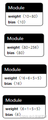
self.label_result.setText(str(predicted.item()))(5)保存后的网络模型可视化
浏览器输入链接:netron

点击按钮,打开保存的.pt文件,就可以显示网络机构
例:
(6)训练过程可视化
python
def visualize(train_loss,val_loss,val_acc):
    train_loss = np.array(train_loss)
    val_loss = np.array(val_loss)
    val_acc = np.array(val_acc)
    plt.grid(True)
    plt.xlabel("epoch")
    plt.ylabel("value")
    plt.title("train_loss and valid_acc")
    plt.plot(np.arange(len(val_acc)),val_acc, label=r"valid_acc",c="g")
    plt.plot(np.arange(len(train_loss)),train_loss,label=r"train_loss",c="r")
    plt.legend()
    plt.savefig("K:\\a.png")

visualize(train_loss_list,valid_loss_list,valid_accuracy_list)
(7)显示彩色图片
问题1:TypeError: Invalid shape (3, 224, 224) for image data
①灰色图片
python
img_label_list=list(zip(img,label))
for i,(img,label) in enumerate(img_label_list):
    nimg=np.array(img)
    nimg=np.squeeze(nimg)
    plt.subplot(8,8,i+1)
    plt.title(str(label.item()))
    plt.imshow(nimg)
    plt.axis('off')
plt.show()
②彩色图片
python
img_label_list=list(zip(img,label))
for i,(img,label) in enumerate(img_label_list):
    nimg=img.transpose(0, 2)  彩色图像是3*n*n需要先将3移到最后!
    nimg=nimg.numpy()
    plt.subplot(5,5,i+1)
    plt.title(str(label.item()))
    plt.imshow(nimg)
    plt.axis('off')
plt.show() 问题2:Clipping input data to the valid range for imshow with RGB data ([0..1] for floats or [0..255] for integers).
matplotlib.pyplot.imshow()函数在处理灰度图像时,自动将其值做归一化处理而在处理彩色图像时则不会,而是将浮点值变换至[0,1],整数值变换到[0, 255]范围
(8)每次卷积后特征图显示
需要先修改transform:
python
transform=transforms.Compose([
                              transforms.ToTensor(),   #转换成张量
                              transforms.Normalize(mean=[0.485,0.456,0.406],
                                                   std=[0.229,0.224,0.225])
                            ])
python
#保存数据集一张图像
imgs,labels=next(iter(train_dl))
img_label_list=list(zip(imgs,labels))
for i,(img,label) in enumerate(img_label_list):
    nimg=img.transpose(0, 2)
    nimg=nimg.numpy()
    plt.imshow(nimg)
    plt.axis('off')
    plt.savefig('1.png')
    if i==0:
        break

# 传入图片
from PIL import Image

image=Image.open(str(r'1.png')).convert('RGB')
image=transform(image)
print('\n输入图尺寸:{}'.format(image.shape))

image=image.unsqueeze(0)
image=image.to(device)

# 计算卷积个数
model_weights=[] #卷积层参数
conv_layers=[]   #卷积层本身
model_children=list(model.children())
counter=0        #卷积层个数
for i in range(len(model_children)):
    if type(model_children[i])==nn.Conv2d:
        counter+=1
        model_weights.append(model_children[i].weight)
        conv_layers.append(model_children[i])
    elif type(model_children[i])==nn.Sequential:
        for j in range(len(model_children[i])):
            for child in model_children[i][j].children():
                if type(child)==nn.Conv2d:
                    counter+=1
                    model_weights.append(child.weight)
                    conv_layer.append(child)

outputs=[]
names=[]
for layer in conv_layers[0:]:
    image=layer(image)
    outputs.append(image)
    names.append(str(layer))
print('特征图尺寸:{}'.format(outputs[1].shape))

#具体绘制特征图
processed=[]
for feature_map in outputs:
    feature_map=feature_map.squeeze(0)
    gray_scale=torch.sum(feature_map,0)
    gray_scale=gray_scale/feature_map.shape[0]
    processed.append(gray_scale.data.cpu().numpy())
fig=plt.figure()

for i in range(len(processed)):
    a=fig.add_subplot(5,4,i+1)
    imgplot=plt.imshow(processed[i])
    a.axis('off')
    a.set_title(names[i].split('(')[0],fontsize=10)
plt.savefig('feature_map.png',bbox_inches='tight')
print('over!')
(9)运行过程中忽视警告
python
import warnings
warnings.filterwarnings("ignore")