目录
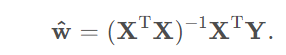
1.最小二乘法:
平面几何表达直线(两个系数):
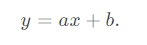
重新命名变量:
强行加一个x0=1:
向量表达:
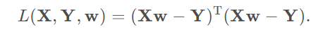
2.损失函数:
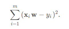
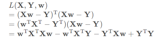
矩阵表达:
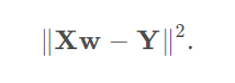
矩阵展开:
推导:
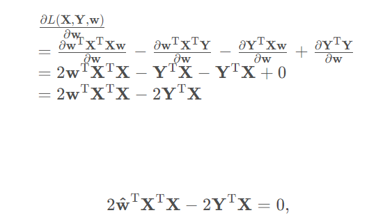
为最小化该函数, 应对w求导, 且其结果为0。
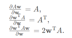
根据矩阵求导法则:
于是有:
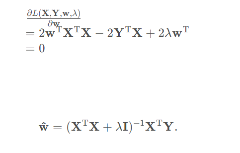
解得:
在我们上面求出来的最小二乘法求损失函数最小值的时候,求出来的值,但是有个问题,如多数剧中的
如果是奇异阵无法求逆该怎么办。下面将岭回归解决:
1.岭回归
- 动机: 奇异矩阵无法求逆
- 方案: 在对角线上加常数
损失函数:
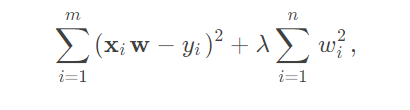
其中, 后半部分是正则项.
矩阵化的展开式:

求导:
1.1代码示例
python
# 导入必要的库
import numpy as np
import matplotlib
matplotlib.use('TkAgg')
import matplotlib.pyplot as plt
from sklearn.linear_model import Ridge
from sklearn.model_selection import train_test_split
from sklearn.metrics import mean_squared_error

# 创建示例数据集
np.random.seed(0)
X = np.random.rand(100, 10)  # 100个样本,10个特征
y = 2 * X[:, 0] + 3 * X[:, 1] + np.random.randn(100)  # 构造线性关系,并添加噪声

# 将数据集划分为训练集和测试集
X_train, X_test, y_train, y_test = train_test_split(X, y, test_size=0.2, random_state=42)

# 定义岭回归模型
ridge = Ridge(alpha=1.0)  # alpha为岭参数,默认为1.0

# 在训练集上训练模型
ridge.fit(X_train, y_train)

# 在测试集上进行预测
y_pred = ridge.predict(X_test)

# 计算均方误差(MSE)作为性能评估指标
mse = mean_squared_error(y_test, y_pred)
print("岭回归模型的均方误差为:", mse)

# 绘制预测值与真实值的对比图


plt.figure(figsize=(8, 6))
plt.scatter(y_test, y_pred, color='blue')
plt.plot([y_test.min(), y_test.max()], [y_test.min(), y_test.max()], linestyle='--', color='red')
plt.xlabel('True Values')
plt.ylabel('Predictions')
plt.title('True vs. Predicted Values (Ridge Regression)')
plt.show()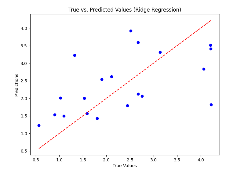
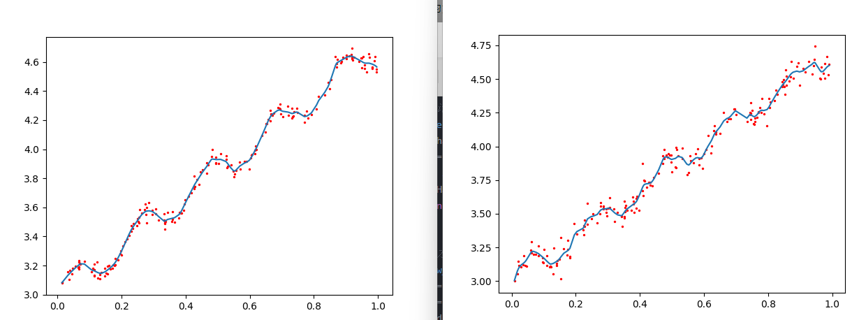
2.局部线性回归
local linear regression
- 动机: 线性回归太粗暴, 在x xx或t tt变化大时不适合
- 方案: 局部加权
当两个样本点的特征向量距离较近时,它们的输出变量通常比较接近,也就是说它们具有相似的性质。现在我们有m 个训练样本点( x 1 , y 1 ) , ( x 2 , y 2 ) , ... , ( x m , y m )构成训练集。那么当我们给一个特征向量x 时,要根据训练集中的信息预测出它的输出变量y ,距离x 越近的训练集中的样本点越应该被重视。换句话说,我们需要给训练集中的每个样本点一个权值,距离x 越近的样本点的权值应该越大,这是赋权的一个原则,那么具体应该如何赋权呢?
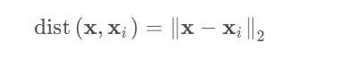
欧氏距离(2范数)是一种常用的度量方法:
高斯核是另外一种度量方法:
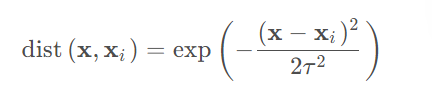
其中,x 为新预测的样本特征数据,x i为训练集的样本特征数据。参数τ控制了权值变化的速率.
损失函数:
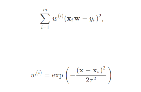
权值有如下性质:

矩阵化展开式: 是对角矩阵
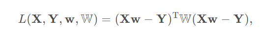
对w求偏导且等于0(损失函数最小):

它比线性回归的式子多了一个对角矩阵W , 因此在W=I时退化为前者.
2.1代码示例
数据集:
ex0.txt:
python
1.000000	0.067732	3.176513
1.000000	0.427810	3.816464
1.000000	0.995731	4.550095
1.000000	0.738336	4.256571
1.000000	0.981083	4.560815
1.000000	0.526171	3.929515
1.000000	0.378887	3.526170
1.000000	0.033859	3.156393
1.000000	0.132791	3.110301
1.000000	0.138306	3.149813
1.000000	0.247809	3.476346
1.000000	0.648270	4.119688
1.000000	0.731209	4.282233
1.000000	0.236833	3.486582
1.000000	0.969788	4.655492
1.000000	0.607492	3.965162
1.000000	0.358622	3.514900
1.000000	0.147846	3.125947
1.000000	0.637820	4.094115
1.000000	0.230372	3.476039
1.000000	0.070237	3.210610
1.000000	0.067154	3.190612
1.000000	0.925577	4.631504
1.000000	0.717733	4.295890
1.000000	0.015371	3.085028
1.000000	0.335070	3.448080
1.000000	0.040486	3.167440
1.000000	0.212575	3.364266
1.000000	0.617218	3.993482
1.000000	0.541196	3.891471
1.000000	0.045353	3.143259
1.000000	0.126762	3.114204
1.000000	0.556486	3.851484
1.000000	0.901144	4.621899
1.000000	0.958476	4.580768
1.000000	0.274561	3.620992
1.000000	0.394396	3.580501
1.000000	0.872480	4.618706
1.000000	0.409932	3.676867
1.000000	0.908969	4.641845
1.000000	0.166819	3.175939
1.000000	0.665016	4.264980
1.000000	0.263727	3.558448
1.000000	0.231214	3.436632
1.000000	0.552928	3.831052
1.000000	0.047744	3.182853
1.000000	0.365746	3.498906
1.000000	0.495002	3.946833
1.000000	0.493466	3.900583
1.000000	0.792101	4.238522
1.000000	0.769660	4.233080
1.000000	0.251821	3.521557
1.000000	0.181951	3.203344
1.000000	0.808177	4.278105
1.000000	0.334116	3.555705
1.000000	0.338630	3.502661
1.000000	0.452584	3.859776
1.000000	0.694770	4.275956
1.000000	0.590902	3.916191
1.000000	0.307928	3.587961
1.000000	0.148364	3.183004
1.000000	0.702180	4.225236
1.000000	0.721544	4.231083
1.000000	0.666886	4.240544
1.000000	0.124931	3.222372
1.000000	0.618286	4.021445
1.000000	0.381086	3.567479
1.000000	0.385643	3.562580
1.000000	0.777175	4.262059
1.000000	0.116089	3.208813
1.000000	0.115487	3.169825
1.000000	0.663510	4.193949
1.000000	0.254884	3.491678
1.000000	0.993888	4.533306
1.000000	0.295434	3.550108
1.000000	0.952523	4.636427
1.000000	0.307047	3.557078
1.000000	0.277261	3.552874
1.000000	0.279101	3.494159
1.000000	0.175724	3.206828
1.000000	0.156383	3.195266
1.000000	0.733165	4.221292
1.000000	0.848142	4.413372
1.000000	0.771184	4.184347
1.000000	0.429492	3.742878
1.000000	0.162176	3.201878
1.000000	0.917064	4.648964
1.000000	0.315044	3.510117
1.000000	0.201473	3.274434
1.000000	0.297038	3.579622
1.000000	0.336647	3.489244
1.000000	0.666109	4.237386
1.000000	0.583888	3.913749
1.000000	0.085031	3.228990
1.000000	0.687006	4.286286
1.000000	0.949655	4.628614
1.000000	0.189912	3.239536
1.000000	0.844027	4.457997
1.000000	0.333288	3.513384
1.000000	0.427035	3.729674
1.000000	0.466369	3.834274
1.000000	0.550659	3.811155
1.000000	0.278213	3.598316
1.000000	0.918769	4.692514
1.000000	0.886555	4.604859
1.000000	0.569488	3.864912
1.000000	0.066379	3.184236
1.000000	0.335751	3.500796
1.000000	0.426863	3.743365
1.000000	0.395746	3.622905
1.000000	0.694221	4.310796
1.000000	0.272760	3.583357
1.000000	0.503495	3.901852
1.000000	0.067119	3.233521
1.000000	0.038326	3.105266
1.000000	0.599122	3.865544
1.000000	0.947054	4.628625
1.000000	0.671279	4.231213
1.000000	0.434811	3.791149
1.000000	0.509381	3.968271
1.000000	0.749442	4.253910
1.000000	0.058014	3.194710
1.000000	0.482978	3.996503
1.000000	0.466776	3.904358
1.000000	0.357767	3.503976
1.000000	0.949123	4.557545
1.000000	0.417320	3.699876
1.000000	0.920461	4.613614
1.000000	0.156433	3.140401
1.000000	0.656662	4.206717
1.000000	0.616418	3.969524
1.000000	0.853428	4.476096
1.000000	0.133295	3.136528
1.000000	0.693007	4.279071
1.000000	0.178449	3.200603
1.000000	0.199526	3.299012
1.000000	0.073224	3.209873
1.000000	0.286515	3.632942
1.000000	0.182026	3.248361
1.000000	0.621523	3.995783
1.000000	0.344584	3.563262
1.000000	0.398556	3.649712
1.000000	0.480369	3.951845
1.000000	0.153350	3.145031
1.000000	0.171846	3.181577
1.000000	0.867082	4.637087
1.000000	0.223855	3.404964
1.000000	0.528301	3.873188
1.000000	0.890192	4.633648
1.000000	0.106352	3.154768
1.000000	0.917886	4.623637
1.000000	0.014855	3.078132
1.000000	0.567682	3.913596
1.000000	0.068854	3.221817
1.000000	0.603535	3.938071
1.000000	0.532050	3.880822
1.000000	0.651362	4.176436
1.000000	0.901225	4.648161
1.000000	0.204337	3.332312
1.000000	0.696081	4.240614
1.000000	0.963924	4.532224
1.000000	0.981390	4.557105
1.000000	0.987911	4.610072
1.000000	0.990947	4.636569
1.000000	0.736021	4.229813
1.000000	0.253574	3.500860
1.000000	0.674722	4.245514
1.000000	0.939368	4.605182
1.000000	0.235419	3.454340
1.000000	0.110521	3.180775
1.000000	0.218023	3.380820
1.000000	0.869778	4.565020
1.000000	0.196830	3.279973
1.000000	0.958178	4.554241
1.000000	0.972673	4.633520
1.000000	0.745797	4.281037
1.000000	0.445674	3.844426
1.000000	0.470557	3.891601
1.000000	0.549236	3.849728
1.000000	0.335691	3.492215
1.000000	0.884739	4.592374
1.000000	0.918916	4.632025
1.000000	0.441815	3.756750
1.000000	0.116598	3.133555
1.000000	0.359274	3.567919
1.000000	0.814811	4.363382
1.000000	0.387125	3.560165
1.000000	0.982243	4.564305
1.000000	0.780880	4.215055
1.000000	0.652565	4.174999
1.000000	0.870030	4.586640
1.000000	0.604755	3.960008
1.000000	0.255212	3.529963
1.000000	0.730546	4.213412
1.000000	0.493829	3.908685
1.000000	0.257017	3.585821
1.000000	0.833735	4.374394
1.000000	0.070095	3.213817
1.000000	0.527070	3.952681
1.000000	0.116163	3.129283
ex1.txt:
python
1.000000	0.635975	4.093119
1.000000	0.552438	3.804358
1.000000	0.855922	4.456531
1.000000	0.083386	3.187049
1.000000	0.975802	4.506176
1.000000	0.181269	3.171914
1.000000	0.129156	3.053996
1.000000	0.605648	3.974659
1.000000	0.301625	3.542525
1.000000	0.698805	4.234199
1.000000	0.226419	3.405937
1.000000	0.519290	3.932469
1.000000	0.354424	3.514051
1.000000	0.118380	3.105317
1.000000	0.512811	3.843351
1.000000	0.236795	3.576074
1.000000	0.353509	3.544471
1.000000	0.481447	3.934625
1.000000	0.060509	3.228226
1.000000	0.174090	3.300232
1.000000	0.806818	4.331785
1.000000	0.531462	3.908166
1.000000	0.853167	4.386918
1.000000	0.304804	3.617260
1.000000	0.612021	4.082411
1.000000	0.620880	3.949470
1.000000	0.580245	3.984041
1.000000	0.742443	4.251907
1.000000	0.110770	3.115214
1.000000	0.742687	4.234319
1.000000	0.574390	3.947544
1.000000	0.986378	4.532519
1.000000	0.294867	3.510392
1.000000	0.472125	3.927832
1.000000	0.872321	4.631825
1.000000	0.843537	4.482263
1.000000	0.864577	4.487656
1.000000	0.341874	3.486371
1.000000	0.097980	3.137514
1.000000	0.757874	4.212660
1.000000	0.877656	4.506268
1.000000	0.457993	3.800973
1.000000	0.475341	3.975979
1.000000	0.848391	4.494447
1.000000	0.746059	4.244715
1.000000	0.153462	3.019251
1.000000	0.694256	4.277945
1.000000	0.498712	3.812414
1.000000	0.023580	3.116973
1.000000	0.976826	4.617363
1.000000	0.624004	4.005158
1.000000	0.472220	3.874188
1.000000	0.390551	3.630228
1.000000	0.021349	3.145849
1.000000	0.173488	3.192618
1.000000	0.971028	4.540226
1.000000	0.595302	3.835879
1.000000	0.097638	3.141948
1.000000	0.745972	4.323316
1.000000	0.676390	4.204829
1.000000	0.488949	3.946710
1.000000	0.982873	4.666332
1.000000	0.296060	3.482348
1.000000	0.228008	3.451286
1.000000	0.671059	4.186388
1.000000	0.379419	3.595223
1.000000	0.285170	3.534446
1.000000	0.236314	3.420891
1.000000	0.629803	4.115553
1.000000	0.770272	4.257463
1.000000	0.493052	3.934798
1.000000	0.631592	4.154963
1.000000	0.965676	4.587470
1.000000	0.598675	3.944766
1.000000	0.351997	3.480517
1.000000	0.342001	3.481382
1.000000	0.661424	4.253286
1.000000	0.140912	3.131670
1.000000	0.373574	3.527099
1.000000	0.223166	3.378051
1.000000	0.908785	4.578960
1.000000	0.915102	4.551773
1.000000	0.410940	3.634259
1.000000	0.754921	4.167016
1.000000	0.764453	4.217570
1.000000	0.101534	3.237201
1.000000	0.780368	4.353163
1.000000	0.819868	4.342184
1.000000	0.173990	3.236950
1.000000	0.330472	3.509404
1.000000	0.162656	3.242535
1.000000	0.476283	3.907937
1.000000	0.636391	4.108455
1.000000	0.758737	4.181959
1.000000	0.778372	4.251103
1.000000	0.936287	4.538462
1.000000	0.510904	3.848193
1.000000	0.515737	3.974757
1.000000	0.437823	3.708323
1.000000	0.828607	4.385210
1.000000	0.556100	3.927788
1.000000	0.038209	3.187881
1.000000	0.321993	3.444542
1.000000	0.067288	3.199263
1.000000	0.774989	4.285745
1.000000	0.566077	3.878557
1.000000	0.796314	4.155745
1.000000	0.746600	4.197772
1.000000	0.360778	3.524928
1.000000	0.397321	3.525692
1.000000	0.062142	3.211318
1.000000	0.379250	3.570495
1.000000	0.248238	3.462431
1.000000	0.682561	4.206177
1.000000	0.355393	3.562322
1.000000	0.889051	4.595215
1.000000	0.733806	4.182694
1.000000	0.153949	3.320695
1.000000	0.036104	3.122670
1.000000	0.388577	3.541312
1.000000	0.274481	3.502135
1.000000	0.319401	3.537559
1.000000	0.431653	3.712609
1.000000	0.960398	4.504875
1.000000	0.083660	3.262164
1.000000	0.122098	3.105583
1.000000	0.415299	3.742634
1.000000	0.854192	4.566589
1.000000	0.925574	4.630884
1.000000	0.109306	3.190539
1.000000	0.805161	4.289105
1.000000	0.344474	3.406602
1.000000	0.769116	4.251899
1.000000	0.182003	3.183214
1.000000	0.225972	3.342508
1.000000	0.413088	3.747926
1.000000	0.964444	4.499998
1.000000	0.203334	3.350089
1.000000	0.285574	3.539554
1.000000	0.850209	4.443465
1.000000	0.061561	3.290370
1.000000	0.426935	3.733302
1.000000	0.389376	3.614803
1.000000	0.096918	3.175132
1.000000	0.148938	3.164284
1.000000	0.893738	4.619629
1.000000	0.195527	3.426648
1.000000	0.407248	3.670722
1.000000	0.224357	3.412571
1.000000	0.045963	3.110330
1.000000	0.944647	4.647928
1.000000	0.756552	4.164515
1.000000	0.432098	3.730603
1.000000	0.990511	4.609868
1.000000	0.649699	4.094111
1.000000	0.584879	3.907636
1.000000	0.785934	4.240814
1.000000	0.029945	3.106915
1.000000	0.075747	3.201181
1.000000	0.408408	3.872302
1.000000	0.583851	3.860890
1.000000	0.497759	3.884108
1.000000	0.421301	3.696816
1.000000	0.140320	3.114540
1.000000	0.546465	3.791233
1.000000	0.843181	4.443487
1.000000	0.295390	3.535337
1.000000	0.825059	4.417975
1.000000	0.946343	4.742471
1.000000	0.350404	3.470964
1.000000	0.042787	3.113381
1.000000	0.352487	3.594600
1.000000	0.590736	3.914875
1.000000	0.120748	3.108492
1.000000	0.143140	3.152725
1.000000	0.511926	3.994118
1.000000	0.496358	3.933417
1.000000	0.382802	3.510829
1.000000	0.252464	3.498402
1.000000	0.845894	4.460441
1.000000	0.132023	3.245277
1.000000	0.442301	3.771067
1.000000	0.266889	3.434771
1.000000	0.008575	2.999612
1.000000	0.897632	4.454221
1.000000	0.533171	3.985348
1.000000	0.285243	3.557982
1.000000	0.377258	3.625972
1.000000	0.486995	3.922226
1.000000	0.305993	3.547421
1.000000	0.277528	3.580944
1.000000	0.750899	4.268081
1.000000	0.694756	4.278096
1.000000	0.870158	4.517640
1.000000	0.276457	3.555461
1.000000	0.017761	3.055026
1.000000	0.802046	4.354819
1.000000	0.559275	3.894387
1.000000	0.941305	4.597773
1.000000	0.856877	4.523616
1.加载数据集
python
# 定义一个函数用于加载数据集
def loadDataSet(fileName):
    # 计算特征数量,通过读取文件的第一行并计算分隔符'\t'的数量减去1
    numFeat = len(open(fileName).readline().split('\t')) - 1
    # 初始化数据矩阵和标签矩阵
    dataMat = []; labelMat = []
    # 打开文件
    fr = open(fileName)
    # 逐行读取文件内容
    for line in fr.readlines():
        # 初始化当前行的特征列表
        lineArr =[]
        # 去除行首尾的空白字符,并按'\t'分割字符串
        curLine = line.strip().split('\t')
        # 遍历特征,将每个特征转换为浮点数并添加到特征列表中
        for i in range(numFeat):
            lineArr.append(float(curLine[i]))
        # 将特征列表添加到数据矩阵中
        dataMat.append(lineArr)
        # 将标签(最后一列)添加到标签矩阵中
        labelMat.append(float(curLine[-1]))
    # 返回数据矩阵和标签矩阵
    return dataMat,labelMat
2.局部加权线性回归
python
from numpy import *
from numpy.linalg import linalg

# 定义局部加权线性回归函数
def lwlr(testPoint, xArr, yArr, k=1.0):
    # 将输入数据转换为矩阵形式
    xMat = np.asmatrix(xArr)
    yMat = np.asmatrix(yArr).T
    # 获取数据点的数量
    m = shape(xMat)[0]
    # 初始化权重矩阵为单位矩阵
    weights =np.asmatrix(eye((m)))
    # 计算每个数据点的权重
    for j in range(m):
        # 计算测试点与每个数据点的差值
        diffMat = testPoint - xMat[j, :]
        # 计算权重,并赋值给权重矩阵的对角线元素
        weights[j, j] = exp(diffMat * diffMat.T / (-2.0 * k**2))
    # 计算X的转置乘以权重乘以X
    xTx = xMat.T * (weights * xMat)
    # 检查矩阵是否可逆
    if linalg.det(xTx) == 0.0:
        print("This matrix is singular, cannot do inverse")
        return
    # 计算回归系数
    ws = xTx.I * (xMat.T * (weights * yMat))
    # 返回测试点的预测结果
    return testPoint * ws
3.画图
python
#对所有点计算回归值
def lwlrTest(testArr,xArr,yArr,k=1): #计算所有数据点的预测回归值,默认k=1,即完全线性回归
    m = shape(testArr)[0]
    yHat = zeros(m)
    for i in range(m):
        yHat[i] = lwlr(testArr[i],xArr,yArr,k)
    return yHat


#画出回归方程
def plot_w_figure(xArr,yArr,k=1):
    yHat = lwlrTest(xArr,xArr,yArr,k)
    xMat = np.asmatrix(xArr)
    srtInd = xMat[:,1].argsort(0)#将输入值x从大到小排序并返回索引
    xSort = xMat[srtInd][:,0,:]
    # print(xSort.shape)
    # print(xSort)
    fig = plt.figure()
    ax = fig.add_subplot(111)
    ax.plot(xSort[:,1],yHat[srtInd])#绘制预测点
    ax.scatter(xMat[:,1].flatten().A[0],np.asmatrix(yArr).T.flatten().A[0],s=2,c='red')#绘制初始数据点
    plt.show()


xArr,yArr=loadDataSet('C:\pythonProject\机器学习\回归算法\局部线性回归\ex0.txt')
xArr1,yArr1=loadDataSet('C:\pythonProject\机器学习\回归算法\局部线性回归\ex1.txt')
plot_w_figure(xArr,yArr,k=0.01)
plot_w_figure(xArr1,yArr1,k=0.01)