《数字图像处理》第三章 3.8 基于模糊技术的图像强度变换与空间滤波学习笔记

请注意:笔记内容片面粗浅，请读者批判着阅读！

在传统图像处理中，灰度变换 和空间滤波 通常采用确定性数学方法（如直方图均衡化、均值滤波等）。但当面对图像中的不确定性 （如光照不均、噪声模糊性、边缘过渡区）时，模糊逻辑（Fuzzy Logic）展现出了独特优势。

一、模糊理论基础

1.1 模糊集合与隶属函数

模糊集合突破了传统二值逻辑（0或1），允许元素以隶属度（0到1之间的值）表示归属程度。例如在灰度图像中，可将像素分为"暗"、"中灰"、"亮"三个模糊集合，通过高斯型或三角形隶属函数量化其归属程度。

python 复制代码

import numpy as np
import skfuzzy as fuzz
import matplotlib.pyplot as plt

# 定义灰度值范围 [0,255]
gray_levels = np.arange(0, 256, 1)

# 创建三个模糊集合的隶属函数
dark = fuzz.gaussmf(gray_levels, 50, 30)     # 中心50，标准差30
medium = fuzz.gaussmf(gray_levels, 128, 40)  
bright = fuzz.gaussmf(gray_levels, 200, 30)

# 可视化
plt.figure()
plt.plot(gray_levels, dark, 'b', linewidth=1.5, label='Dark')
plt.plot(gray_levels, medium, 'g', linewidth=1.5, label='Medium')
plt.plot(gray_levels, bright, 'r', linewidth=1.5, label='Bright')
plt.legend()
plt.title('Fuzzy Membership Functions')
plt.show()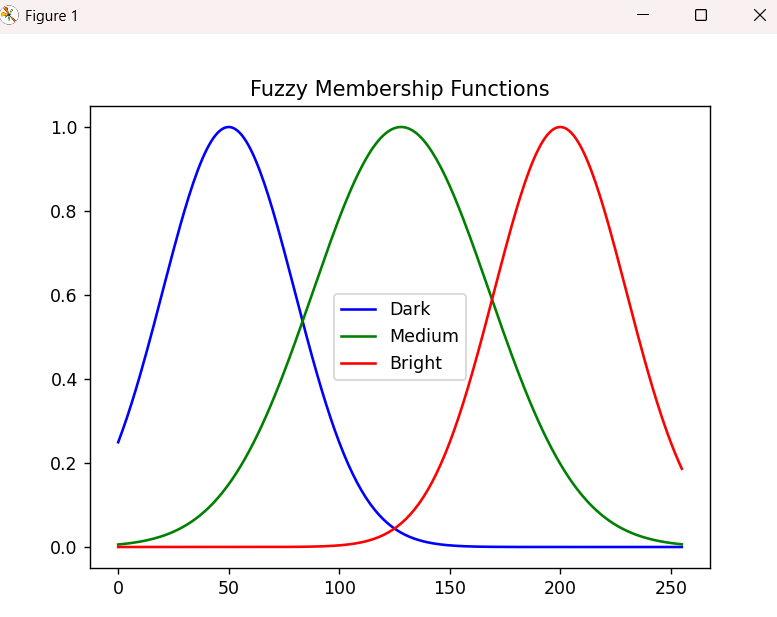

1.2 模糊规则库

基于专家经验构建推理规则，例如：

规则1：如果像素属于"暗"区域，则增强其对比度；
规则2：如果像素属于"亮"且邻域差异大，则进行锐化。

二、模糊强度变换应用

根据应用场景设计逻辑规则：

python 复制代码

规则1：IF 像素属于Dark → THEN 输出更暗（如原值×0.8）  
规则2：IF 像素属于Gray → THEN 保持原值  
规则3：IF 像素属于Bright → THEN 输出更亮（如原值×1.2）

2.1 自适应对比度增强

传统直方图均衡化可能过度增强噪声，而模糊方法通过动态调整增强强度实现更自然的变换。
实现步骤：

计算每个像素的暗/中/亮隶属度
根据规则计算增强权重
合成新像素值

python 复制代码

import cv2
from skimage import data, color
import numpy as np
import matplotlib.pyplot as plt
import skfuzzy as fuzz


# 感受一下即可，我已经尽力了。。。
def fuzzy_contrast_enhance(img):
    # 灰度化
    gray = color.rgb2gray(img) * 255
    enhanced = np.zeros_like(gray)

    for i in range(gray.shape[0]):
        for j in range(gray.shape[1]):
            # 计算当前像素隶属度
            dark_mf = fuzz.gaussmf(gray[i, j], 50, 30)
            medium_mf = fuzz.gaussmf(gray[i, j], 128, 40)
            bright_mf = fuzz.gaussmf(gray[i, j], 200, 30)

            # 应用规则：暗区线性增强，亮区保持
            new_val = 0.8 * dark_mf * (gray[i, j] * 1.5) + \
                      0.2 * medium_mf * gray[i, j] + \
                      0.1 * bright_mf * gray[i, j]

            enhanced[i, j] = np.clip(new_val, 0, 255)
    return enhanced


img = data.astronaut()

plt.subplot(1, 2, 1)
plt.imshow(img, cmap='gray')
plt.title('Original')
plt.axis('off')

result = fuzzy_contrast_enhance(img)
plt.subplot(1, 2, 2)
plt.imshow(result, cmap='gray')
plt.title('Fuzzy Contrast Enhance')
plt.axis('off')

plt.show()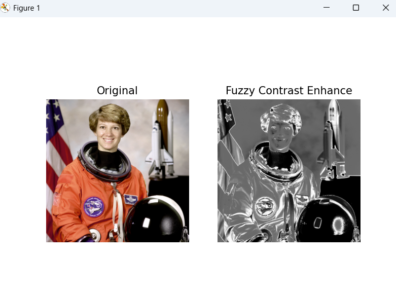

2.2 与传统方法对比

图中展示了模糊增强（右）与直方图均衡化（左）的效果差异，可见模糊方法在保留亮部细节的同时更自然地增强了暗部。

三、模糊空间滤波设计

3.1 边缘检测滤波器

传统Sobel算子对噪声敏感，而模糊滤波器可通过分析邻域灰度差异的隶属度实现鲁棒检测。

设计步骤：

定义邻域差异的模糊集合（小/中/大）
构建规则："若差异大，则标记为边缘"
去模糊化输出边缘强度

python 复制代码

import numpy as np
import skfuzzy as fuzz
from scipy.ndimage import convolve
from skimage import data, color
import matplotlib.pyplot as plt


def fuzzy_edge_detection(img):
    """基于模糊逻辑的边缘检测"""
    # 输入处理
    if len(img.shape) == 3:
        gray = color.rgb2gray(img) * 255
    else:
        gray = img.astype(float)
    gray = np.clip(gray, 0, 255).astype(np.uint8)

    # Sobel梯度计算
    sobel_x = np.array([[-1, 0, 1], [-2, 0, 2], [-1, 0, 1]])
    sobel_y = np.array([[1, 2, 1], [0, 0, 0], [-1, -2, -1]])
    grad_x = convolve(gray, sobel_x)
    grad_y = convolve(gray, sobel_y)
    gradient = np.sqrt(grad_x ** 2 + grad_y ** 2)

    # 梯度幅值归一化
    gradient = (gradient / gradient.max()) * 255  # 归一化到[0,255]
    gradient = gradient.astype(np.uint8)  # 转换为整数

    # 定义梯度隶属函数
    grad_levels = np.arange(0, 256)
    low = fuzz.trapmf(grad_levels, [0, 20, 60, 100])  # 低梯度过渡区
    high = fuzz.trapmf(grad_levels, [60, 100, 255, 255])  # 高梯度响应区

    # 预计算隶属度
    high_mf = fuzz.interp_membership(grad_levels, high, grad_levels)

    # 应用模糊规则
    edge_strength = high_mf[gradient] * 255

    return edge_strength.astype(np.uint8)


if __name__ == "__main__":
    img = data.camera()
    edges = fuzzy_edge_detection(img)

    plt.figure(figsize=(12, 6))
    plt.subplot(1, 2, 1)
    plt.imshow(img, cmap='gray')
    plt.title('Original')
    plt.axis('off')

    plt.subplot(1, 2, 2)
    plt.imshow(edges, cmap='gray', vmin=0, vmax=255)  # 强制显示范围
    plt.title('Fuzzy Edges (Fixed)')
    plt.axis('off')
    plt.show()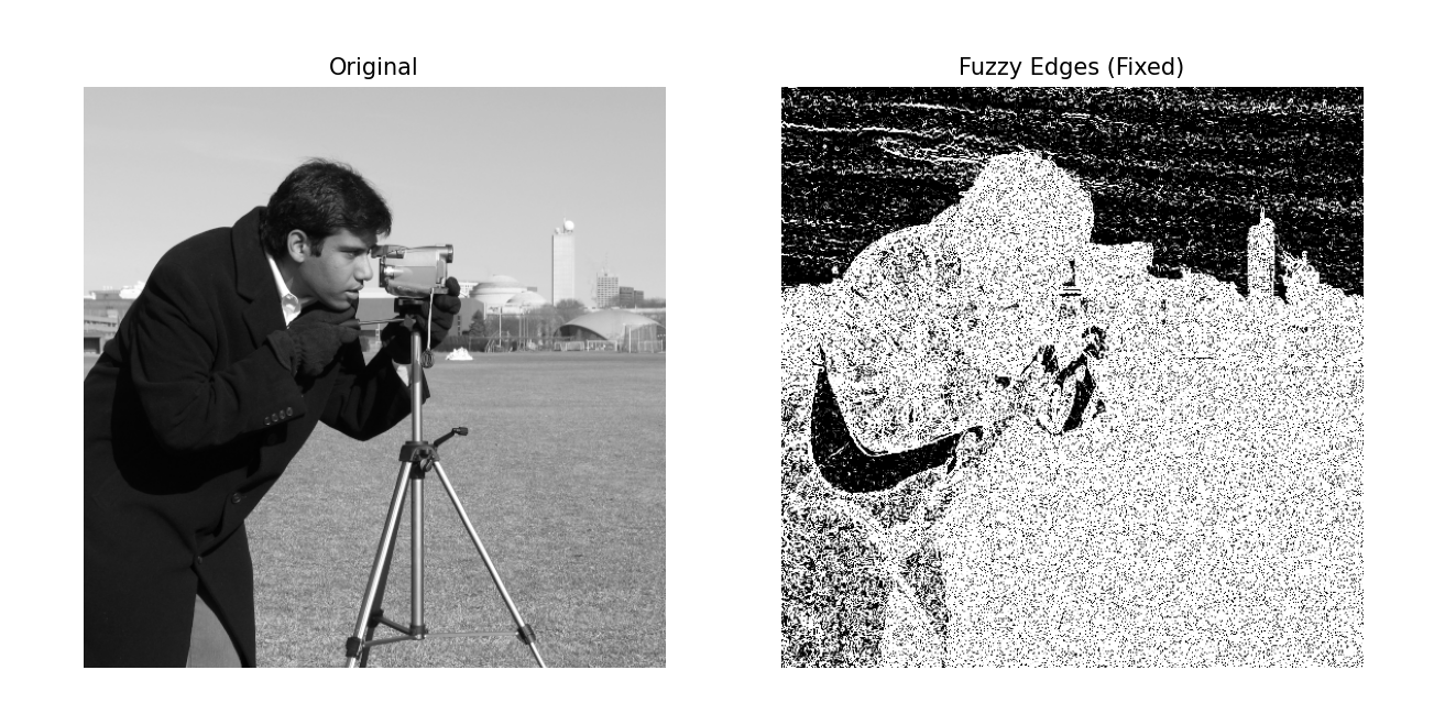

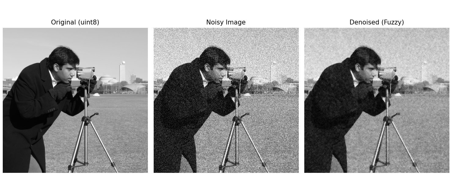
3.2 去噪滤波器

通过分析邻域像素的相似度隶属度，动态调整滤波强度：

python 复制代码

import numpy as np
from skimage import data, util, color
import matplotlib.pyplot as plt
from skimage.util import view_as_windows


def fuzzy_denoise(img, window_size=5, sigma=30):
    # 强制转为浮点灰度图
    if len(img.shape) == 3:
        img = color.rgb2gray(img) * 255
    img = img.astype(np.float32)

    # 镜像填充
    pad = window_size // 2
    padded = np.pad(img, pad, mode='reflect')

    # 向量化窗口操作
    windows = view_as_windows(padded, (window_size, window_size))
    h, w = img.shape
    denoised = np.zeros_like(img)

    for i in range(h):
        for j in range(w):
            window = windows[i, j]
            center = window[pad, pad]

            # 计算相似度（优化防零除）
            diffs = np.abs(window - center)
            similarity = np.exp(-diffs / sigma)  # 高斯型隶属函数
            sum_weights = np.sum(similarity) + 1e-6  # 确保分母非零

            denoised[i, j] = np.sum(window * similarity) / sum_weights

    # 归一化并转为uint8
    denoised = np.clip(denoised, 0, 255).astype(np.uint8)
    return denoised


if __name__ == "__main__":
    # 生成有效测试数据
    original = data.camera().astype(np.uint8)  # 确保输入为uint8
    noisy = util.random_noise(original, mode='gaussian', var=0.02)  # 生成[0,1]浮点
    noisy = (noisy * 255).astype(np.uint8)  # 正确转换为uint8

    # 去噪处理
    denoised = fuzzy_denoise(noisy, sigma=40, window_size=7)

    # 正确显示图像
    plt.figure(figsize=(12, 6))

    plt.subplot(1, 3, 1)
    plt.imshow(original, cmap='gray', vmin=0, vmax=255)
    plt.title('Original (uint8)')
    plt.axis('off')

    plt.subplot(1, 3, 2)
    plt.imshow(noisy, cmap='gray', vmin=0, vmax=255)
    plt.title('Noisy Image')
    plt.axis('off')

    plt.subplot(1, 3, 3)
    plt.imshow(denoised, cmap='gray', vmin=0, vmax=255)
    plt.title('Denoised (Fuzzy)')
    plt.axis('off')

    plt.tight_layout()
    plt.show()