Python----机器学习（KNN：使用数学方法实现KNN）

一、原理

以下是K最近邻（K-Nearest Neighbors，简称KNN）算法的基本流程，用于对给定点进行分类预测。

获得要预测的点 point_predict 。
计算训练点集 point_set_train 中各点到要预测的点表 l ist_L2_distance 。
对 point_predict 的L2距离，得到距离列 list_L2_distance 进行排序，得到排序后的索引值列表 list_index_ascend 。
获取超参数 k，表示选择最近邻的个数。
从 list_index_ascend 中取出前 k 个距离最小的索引值，得到对应的训练点集中的点构成的列表 l ist_k_th 。
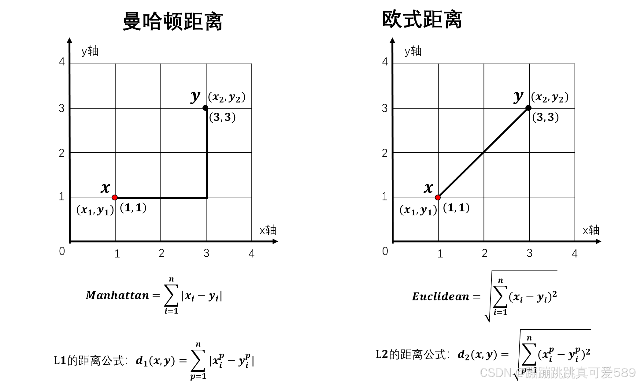
从 list_k_th 中计算各点到要预测的点 point_predict 的L2距离列表，并找到最短距离对应的训练点的标签 label_L2_distance_min ，即为要预测的点的标签。

这个过程基于KNN算法，通过比较新点与训练集中点的距离来决定新点所属的类别。在这里，超参数 k 决定了用于预测的最近邻点的数量。整个过程的关键是计算距离并选择最近邻的点，然后通过这些最近邻的点的标签来确定新点的分类。

导入模块

python 复制代码

import numpy as np
from matplotlib import pyplot as plt
from collections import  Counter

1、定义数据集和测试点

python 复制代码

# 定义三个点集
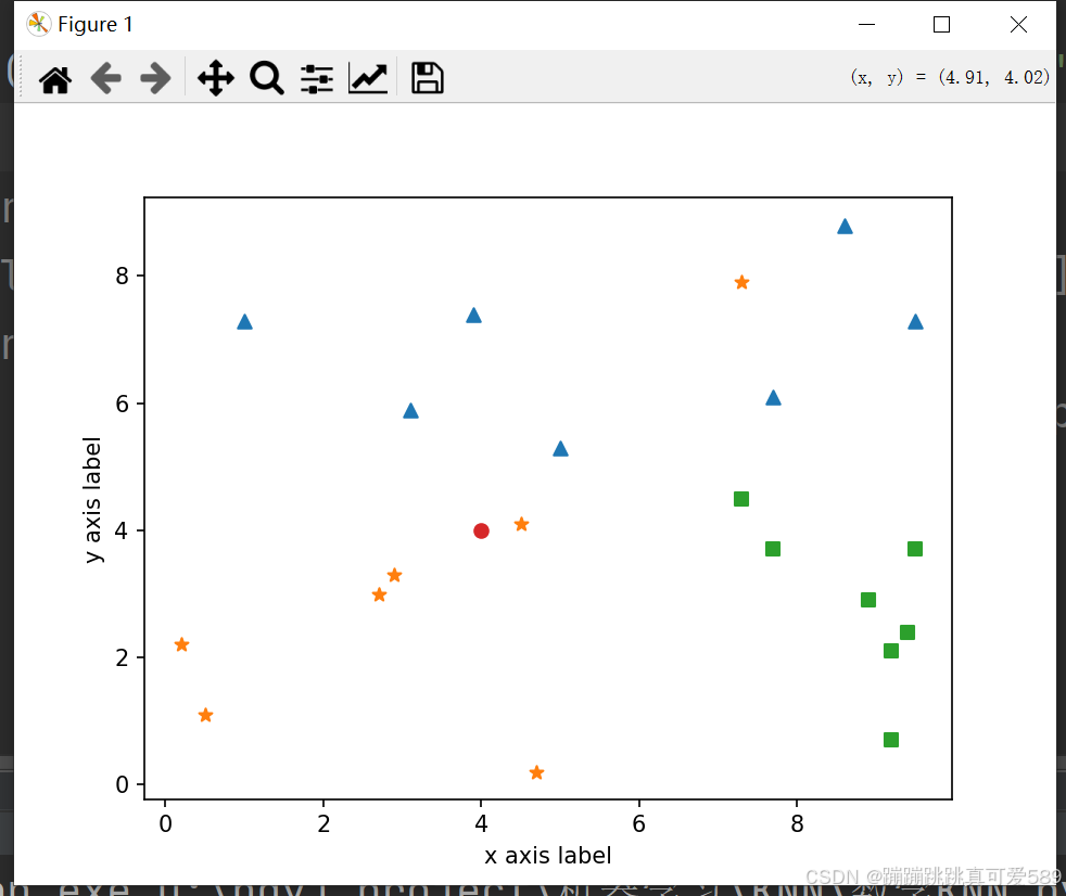
point1 = [[7.7, 6.1], [3.1, 5.9], [8.6, 8.8], [9.5, 7.3], [3.9, 7.4], [5.0, 5.3], [1.0, 7.3]]
point2 = [[0.2, 2.2], [4.5, 4.1], [0.5, 1.1], [2.7, 3.0], [4.7, 0.2], [2.9, 3.3], [7.3, 7.9]]
point3 = [[9.2, 0.7], [9.2, 2.1], [7.3, 4.5], [8.9, 2.9], [9.5, 3.7], [7.7, 3.7], [9.4, 2.4]]

# 合并数据集的特征
np_train_data=np.concatenate(np.array((point1,point2,point3)))

# 生成对应的标签
np_train_label=np.array([0]*7+[1]*7+[2]*7)

#定义一个测试点坐标
predict_point=np.array([4,4])

2、定义K的值

python 复制代码

K=3

3、求距离，获得最短距离、最短距离对应的点的坐标楚

python 复制代码

distance=np.sqrt(np.sum((predict_point-np_train_data)**2,axis=1))

distance_index=np.argsort(distance)

nearest_index=distance_index[:K]

nearest_points=[]
nearest_distance=[]
nearest_label=[]
#拿到前K个点的对应的坐标和距离
for i in nearest_index:
    nearest_points.append(np_train_data[i])
    nearest_distance.append(distance[i])
    nearest_label.append(np_train_label[i])

counter=Counter(nearest_label)

4、绘制

python 复制代码

plt.xlabel("x axis label")
plt.ylabel("y axis label")
plt.scatter(np_train_data[np_train_label==0,0],np_train_data[np_train_label==0,1],marker='^')
plt.scatter(np_train_data[np_train_label==1,0],np_train_data[np_train_label==1,1],marker='*')
plt.scatter(np_train_data[np_train_label==2,0],np_train_data[np_train_label==2,1],marker='s')

plt.scatter(predict_point[0],predict_point[1],marker='o')

for i in range(K):
    plt.plot([predict_point[0],nearest_points[i][0]],[predict_point[1],nearest_points[i][1]])
    plt.annotate(f'{nearest_distance[i]:2.2f}',
                 xy = ((predict_point[0] + nearest_points[i][0]) / 2,(predict_point[1] + nearest_points[i][1]) / 2))

plt.show()

完整代码

python 复制代码

import numpy as np  # 导入 NumPy 库用于数值计算  
from matplotlib import pyplot as plt  # 导入 Matplotlib 库用于数据可视化  
from collections import Counter  # 导入 Counter 以便于统计标签出现频次  

# 1、定义数据集和测试点  
# 定义三个点集（表示不同类别的数据点）  
point1 = [[7.7, 6.1], [3.1, 5.9], [8.6, 8.8], [9.5, 7.3], [3.9, 7.4], [5.0, 5.3], [1.0, 7.3]]  # 类别 0 的点  
point2 = [[0.2, 2.2], [4.5, 4.1], [0.5, 1.1], [2.7, 3.0], [4.7, 0.2], [2.9, 3.3], [7.3, 7.9]]  # 类别 1 的点  
point3 = [[9.2, 0.7], [9.2, 2.1], [7.3, 4.5], [8.9, 2.9], [9.5, 3.7], [7.7, 3.7], [9.4, 2.4]]  # 类别 2 的点  

# 合并数据集的特征  
np_train_data = np.concatenate(np.array((point1, point2, point3)))  # 将所有点集合并为一个 NumPy 数组  

# 生成对应的标签  
np_train_label = np.array([0] * 7 + [1] * 7 + [2] * 7)  # 创建标签数组，标识每个点所属的类别  

# 定义一个测试点坐标  
predict_point = np.array([4, 4])  # 定义需要预测的点坐标  

# 2、定义 K 的值  
K = 3  # 设置 KNN 中 K 的值为 3，表示考虑最近的 3 个邻居  

# 3、求距离，获得最短距离、最短距离对应的点的坐标  
distance = np.sqrt(np.sum((predict_point - np_train_data) ** 2, axis=1))  # 计算测试点与所有训练点的欧几里得距离  

distance_index = np.argsort(distance)  # 获取按距离升序排列的索引  

nearest_index = distance_index[:K]  # 取出最近的 K 个点的索引  

nearest_points = []  # 存储最近 K 个点的坐标  
nearest_distance = []  # 存储最近 K 个点的距离  
nearest_label = []  # 存储最近 K 个点的标签  

# 拿到前 K 个点的对应的坐标和距离  
for i in nearest_index:  
    nearest_points.append(np_train_data[i])  # 添加最近点的坐标  
    nearest_distance.append(distance[i])  # 添加最近点的距离  
    nearest_label.append(np_train_label[i])  # 添加最近点的标签  

# 统计最近 K 个邻居的标签出现频率  
counter = Counter(nearest_label)  # 计算标签的频率  
print(counter.most_common()[0][0])  # 输出出现频率最高的标签（预测结果）  

# 4、绘制  
plt.xlabel("x axis label")  # x 轴标签  
plt.ylabel("y axis label")  # y 轴标签  
# 绘制类别 0 的数据点（标记为三角形）  
plt.scatter(np_train_data[np_train_label == 0, 0], np_train_data[np_train_label == 0, 1], marker='^')  
# 绘制类别 1 的数据点（标记为星形）  
plt.scatter(np_train_data[np_train_label == 1, 0], np_train_data[np_train_label == 1, 1], marker='*')  
# 绘制类别 2 的数据点（标记为方形）  
plt.scatter(np_train_data[np_train_label == 2, 0], np_train_data[np_train_label == 2, 1], marker='s')  

# 绘制待预测点（标记为圆形）  
plt.scatter(predict_point[0], predict_point[1], marker='o', color='red')  

# 绘制预测点与最近邻居之间的连线  
for i in range(K):  
    plt.plot([predict_point[0], nearest_points[i][0]], [predict_point[1], nearest_points[i][1]], color='grey', linestyle='--')  # 画虚线  
    # 在中间位置添加距离的注释  
    plt.annotate(f'{nearest_distance[i]:2.2f}',   
                 xy=((predict_point[0] + nearest_points[i][0]) / 2, (predict_point[1] + nearest_points[i][1]) / 2))  

plt.show()  # 显示绘图结果

二、库函数

2.1、Counter

该模块实现了专门的容器数据类型，提供了 Python 的通用内置容器

from collections import Counter

是用于计算可哈希对象的子类。它是一个集合，其中元素存储为字典键它们的计数存储为字典值。允许计数为任何整数值，包括零或负计数。该类类似于其他语言中的 bags 或 multisets。

函数	方法
namedtuple()	factory 函数，用于创建具有命名字段的 Tuples 子类
deque	类似列表的容器，两端都有快速的附加和弹出
ChainMap	用于创建多个映射的单个视图的类
Counter	dict 子类，用于对可哈希对象进行计数
OrderedDict	dict 子类，该子类会记住已添加的顺序条目
defaultdict	dict 子类，该子类调用工厂函数来提供缺失值
UserDict	Dictionary 对象的包装器，以便于字典子类化
UserList	包装 list 对象，以便更轻松地进行 list 子类化
UserString	String 对象的包装器，以便更轻松地进行字符串子类化

most_common

返回 n 个最常见元素的列表及其从最常见到最不常见。如果省略 n 或， 则返回 计数器中的所有元素。计数相等的元素按第一个en countered 的顺序排序：None
python 复制代码
Counter('abracadabra').most_common(3)
[('a', 5), ('b', 2), ('r', 2)]

2.2、annotate()

python 复制代码

matplotlib.pyplot.annotate(text, xy, xytext=None, xycoords='data', textcoords=None, arrowprops=None, annotation_clip=None, **kwargs)

方法	描述
text	批注的文本。
xy	要注释的点（x， y）。坐标系已确定由 xycoords 提供。
xytext	放置文本的位置（x， y）。坐标系由 TextCoords 确定。
xycoords	给出 xy 的坐标系。
textcoords	给出 xytext 的坐标系。
arrowprops	用于在定位 xy 和 xytext 。默认为 None，即没有箭头是平局。由于历史原因，有两种不同的方法可以指定箭头，"简单"和"花哨"：
annotation_clip	是否在标注点 xy 位于 Axes 区域之外。 * 如果为 True ，则当 xy 在 xy 之外时，将裁剪注释轴。 * 如果为 False，则将始终绘制注释。 * 如果为 None ，则当 xy 位于 x 之外时，将剪切注释轴和 xycoords 是 'data'。
**kwargs	其他 kwargs 将传递给