Python----计算机视觉处理(Opencv:道路检测之道路透视变换)
Python----计算机视觉处理(Opencv:道路检测之提取车道线)
Python----计算机视觉处理(Opencv:道路检测之车道线拟合)
Python----计算机视觉处理(Opencv:道路检测之车道线显示)
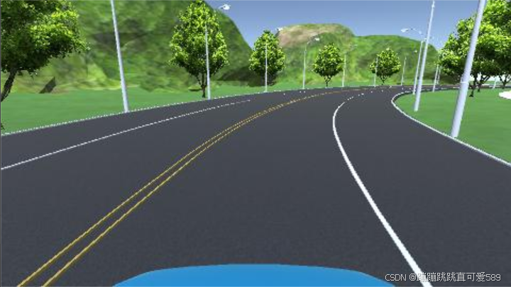
一、透视变换
python
def img_to_wrp(img):
height, width,_= img.shape # 获取输入图像的高度和宽度
# 定义源点(透视变换前的点)
src = np.float32(
[
[width // 2 - 75, height // 2], # 左侧车道线的源点
[width // 2 + 100, height // 2], # 右侧车道线的源点
[0, height], # 底部左侧点
[width, height] # 底部右侧点
]
)
# 定义目标点(透视变换后的点)
dst = np.float32(
[
[0, 0], # 目标左上角
[width, 0], # 目标右上角
[0, height], # 目标左下角
[width, height] # 目标右下角
]
)
# 计算透视变换矩阵
M = cv2.getPerspectiveTransform(src, dst)
# 计算逆透视变换矩阵
W = cv2.getPerspectiveTransform(dst, src)
# 应用透视变换
img_wrp = cv2.warpPerspective(img, M, (width, height), flags=cv2.INTER_LINEAR)
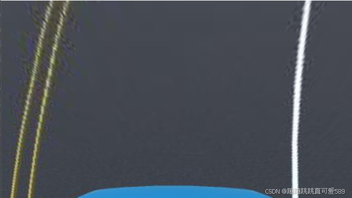
return img_wrp, W # 返回透视变换后的图像和逆变换矩阵这段代码的作用是对输入图像进行透视变换,以便为后续的车道线检测做好准备。
首先,它获取输入图像的高度和宽度,并定义源点(`src`),这些点是透视变换前车道线和底边的具体位置。源点的选取基于图像中车道线的预期位置,以确保透视变换能够有效地将车道区域从图像的视角转变为一个鸟瞰视图。
接下来,定义目标点(`dst`),这些点表示在透视变换后的标准位置,即四个角分别为上左、上右、下左和下右,以便将车道区域展现为一个矩形。
然后,通过 `cv2.getPerspectiveTransform` 计算透视变换矩阵 `M`,同时也计算出逆变换矩阵 `W`。
最后,使用 `cv2.warpPerspective` 应用透视变换,将输入图像转换为新的视角,输出变换后的图像 `img_wrp` 和逆变换矩阵 `W`,这为后续的图像处理和车道线绘制提供了良好的基础。
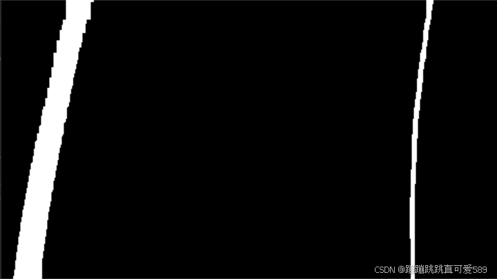
二、提取车道线


python
def img_road_show1(img):
    img_Gaussian = cv2.GaussianBlur(img, (7, 7), sigmaX=1)  # 对图像进行高斯模糊,减少噪声
    img_gray = cv2.cvtColor(img_Gaussian, cv2.COLOR_BGR2GRAY)  # 将模糊后的图像转换为灰度图像
    img_Sobel = cv2.Sobel(img_gray, -1, dx=1, dy=0)  # 使用Sobel算子进行边缘检测,提取水平边缘
    ret, img_threshold = cv2.threshold(img_Sobel, 127, 255, cv2.THRESH_BINARY)  # 二值化处理

    kernel = np.ones((11, 11), np.uint8)  # 创建一个11x11的结构元素
    img_dilate = cv2.dilate(img_threshold, kernel, iterations=2)  # 膨胀操作,增强白色区域
    img_erode = cv2.erode(img_dilate, kernel, iterations=2)  # 腐蚀操作,去除小噪声
    return img_erode  # 返回处理后的图像


def img_road_show2(img):
    # 将图像从BGR颜色空间转换为HLS颜色空间
    img_hls = cv2.cvtColor(img, cv2.COLOR_BGR2HLS)

    # 提取亮度通道
    l_channel = img_hls[:, :, 1]

    # 将亮度通道进行归一化处理
    l_channel = l_channel / np.max(l_channel) * 255

    # 创建与亮度通道同样大小的零数组
    binary_output1 = np.zeros_like(l_channel)

    # 根据亮度阈值提取车道线区域(亮度值范围为220到255)
    binary_output1[(l_channel > 220) & (l_channel < 255)] = 1

    # 提取黄色车道线
    img_lab = cv2.cvtColor(img, cv2.COLOR_BGR2Lab)  # 将图像转换为Lab颜色空间

    # 将图像的下部分设置为黑色,以减少干扰
    img_lab[:, 240:, :] = (0, 0, 0)

    # 提取Lab颜色空间中的蓝色通道
    lab_b = img_lab[:, :, 2]

    # 如果蓝色通道的最大值大于100则归一化处理
    if np.max(lab_b) > 100:
        lab_b = lab_b / np.max(lab_b) * 255

        # 创建与亮度通道同样大小的零数组
    binary_output2 = np.zeros_like(l_channel)

    # 根据蓝色通道的阈值提取车道线区域(蓝色值范围为212到220)
    binary_output2[(lab_b > 212) & (lab_b < 220)] = 1

    # 创建结构元素,用于形态学操作
    kernel = np.ones((15, 15), np.uint8)

    # 对binary_output2进行膨胀操作,以增强车道线
    binary_output2 = cv2.dilate(binary_output2, kernel, iterations=1)

    # 对膨胀后的图像进行两次腐蚀操作,去除小噪声
    binary_output2 = cv2.erode(binary_output2, kernel, iterations=1)
    binary_output2 = cv2.erode(binary_output2, kernel, iterations=1)

    # 创建一个与binary_output1同样大小的零数组
    binary_output = np.zeros_like(binary_output1)

    # 将两个二值输出结合,提取最终车道线区域
    binary_output[(binary_output1 == 1) | (binary_output2 == 1)] = 1

    # 对最终的二值输出进行膨胀处理
    kernel = np.ones((15, 15), np.uint8)
    img_dilate_binary_output = cv2.dilate(binary_output, kernel, iterations=1)

    # 对膨胀后的图像进行腐蚀处理,以便进一步去噪声
    img_erode_binary_output = cv2.erode(img_dilate_binary_output, kernel, iterations=1)

    # 返回最终处理后的图像
    return img_erode_binary_output
这段代码包含两个函数 `img_road_show1` 和 `img_road_show2`,用于处理输入图像并提取车道线区域。
`img_road_show1` 首先对输入图像应用高斯模糊,以减少噪声,然后将其转换为灰度图并使用 Sobel 算子进行边缘检测,以提取水平边缘。接着,进行二值化处理,将边缘图像转为黑白图像。之后,通过形态学操作(膨胀和腐蚀)增强白色区域并去除噪声,最终返回处理后的图像。
`img_road_show2` 则使用 HLS 颜色空间提取亮度通道,并通过阈值划分提取亮度较高的车道线区域。接着,将图像转换为 Lab 颜色空间,提取蓝色通道并进行归一化,依次利用阈值检测提取特定颜色的车道线,然后通过形态学操作去噪。
最终,将两个二值化结果结合,提取出合并的车道线区域,进行再一次的膨胀和腐蚀操作,以确保得到干净的二值图像,最后返回这一处理后的图像,以供后续分析或显示。整体上,这两个函数通过不同的方式(边缘检测和颜色空间分析)强化了车道线的可见性,以便于自动驾驶或图像分析任务。
三、车道线拟合

python
def road_polyfit(img):
    # 获取图像的高度和宽度
    height, width = img.shape
    # 创建一个与输入图像相同大小的RGB图像,用于绘制窗口
    out_img = np.dstack((img, img, img))

    # 计算每一列的白色像素总和,得到直方图
    num_ax0 = np.sum(img, axis=0)

    # 找到直方图左侧和右侧的最高点位置,分别作为车道线的起始点
    img_left_argmax = np.argmax(num_ax0[:width // 2])  # 左侧最高点
    img_right_argmax = np.argmax(num_ax0[width // 2:]) + width // 2  # 右侧最高点

    # 获取图像中所有非零像素的x和y位置
    nonzeroy, nonzerox = np.array(img.nonzero())

    # 定义滑动窗口的数量
    windows_num = 10

    # 定义每个窗口的高度和宽度
    windows_height = height // windows_num
    windows_width = 30

    # 定义在窗口中检测到的白色像素的最小数量
    min_pix = 400

    # 初始化当前窗口的位置,后续会根据检测结果更新
    left_current = img_left_argmax
    right_current = img_right_argmax

    left_pre = left_current  # 记录上一个左侧窗口位置
    right_pre = right_current  # 记录上一个右侧窗口位置

    # 创建空列表以存储左侧和右侧车道线像素的索引
    left_lane_inds = []
    right_lane_inds = []

    # 遍历每个窗口进行车道线检测
    for window in range(windows_num):
        # 计算当前窗口的上边界y坐标
        win_y_high = height - windows_height * (window + 1)
        # 计算当前窗口的下边界y坐标
        win_y_low = height - windows_height * window
        # 计算左侧窗口的左右边界x坐标
        win_x_left_left = left_current - windows_width
        win_x_left_right = left_current + windows_width

        # 计算右侧窗口的左右边界x坐标
        win_x_right_left = right_current - windows_width
        win_x_right_right = right_current + windows_width

        # 在输出图像上绘制当前窗口
        cv2.rectangle(out_img, (win_x_left_left, win_y_high), (win_x_left_right, win_y_low), (0, 255, 0), 2)
        cv2.rectangle(out_img, (win_x_right_left, win_y_high), (win_x_right_right, win_y_low), (0, 255, 0), 2)

        # 找到在当前窗口中符合条件的白色像素索引
        good_left_index = ((nonzeroy >= win_y_high) & (nonzeroy < win_y_low)
                           & (nonzerox >= win_x_left_left) & (nonzerox < win_x_left_right)).nonzero()[0]
        good_right_index = ((nonzeroy >= win_y_high) & (nonzeroy < win_y_low)
                            & (nonzerox >= win_x_right_left) & (nonzerox < win_x_right_right)).nonzero()[0]

        # 将找到的索引添加到列表中
        left_lane_inds.append(good_left_index)
        right_lane_inds.append(good_right_index)

        # 如果找到的左侧像素数量超过阈值,更新左侧窗口位置
        if len(good_left_index) > min_pix:
            left_current = int(np.mean(nonzerox[good_left_index]))
        else:
            # 如果没有找到足够的左侧像素,则根据右侧像素的位置进行偏移
            if len(good_right_index) > min_pix:
                offset = int(np.mean(nonzerox[good_right_index])) - right_pre
                left_current = left_current + offset

                # 如果找到的右侧像素数量超过阈值,更新右侧窗口位置
        if len(good_right_index) > min_pix:
            right_current = int(np.mean(nonzerox[good_right_index]))
        else:
            # 如果没有找到足够的右侧像素,则根据左侧像素的位置进行偏移
            if len(good_left_index) > min_pix:
                offset = int(np.mean(nonzerox[good_left_index])) - left_pre
                right_current = right_current + offset

                # 更新上一个窗口位置
        left_pre = left_current
        right_pre = right_current

        # 将所有的索引连接成一个数组,以便后续提取像素点的坐标
    left_lane_inds = np.concatenate(left_lane_inds)
    right_lane_inds = np.concatenate(right_lane_inds)

    # 提取左侧和右侧车道线像素的位置
    leftx = nonzerox[left_lane_inds]  # 左侧车道线的x坐标
    lefty = nonzeroy[left_lane_inds]  # 左侧车道线的y坐标

    rightx = nonzerox[right_lane_inds]  # 右侧车道线的x坐标
    righty = nonzeroy[right_lane_inds]  # 右侧车道线的y坐标

    # 对左侧和右侧车道线进行多项式拟合,得到拟合曲线的参数
    left_fit = np.polyfit(lefty, leftx, 2)  # 左侧车道线的二次多项式拟合
    right_fit = np.polyfit(righty, rightx, 2)  # 右侧车道线的二次多项式拟合

    # 生成均匀分布的y坐标,用于绘制车道线
    ploty = np.linspace(0, height - 1, height)

    # 根据拟合的多项式计算左侧和右侧车道线的x坐标
    left_fitx = left_fit[0] * ploty ** 2 + left_fit[1] * ploty + left_fit[2]
    right_fitx = right_fit[0] * ploty ** 2 + right_fit[1] * ploty + right_fit[2]

    # 计算中间车道线的位置
    middle_fitx = (left_fitx + right_fitx) // 2

    # 在输出图像上标记车道线像素点
    out_img[lefty, leftx] = [255, 0, 0]  # 左侧车道线
    out_img[righty,rightx]=[0,0,255]# 右侧车道线
    return left_fitx, right_fitx, middle_fitx, ploty
这段代码实现了车道线检测与拟合的功能,主要通过滑动窗口的方法来识别和拟合车道线。首先获取输入图像的高度和宽度,并创建一个与输入图像相同大小的RGB图像用于绘制结果。
接着,通过计算每一列的白色像素总和生成直方图,找到左右车道线的起始点。
然后,定义滑动窗口的数量、每个窗口的高度和宽度,设置检测到的白色像素的最小数量。接下来,遍历每个窗口,绘制窗口并在窗口内检测白色像素的索引。
如果在窗口中找到足够的白色像素,则更新当前窗口的位置;如果没有找到,则根据相邻车道线的像素位置进行调整。
最后,提取所有窗口中检测到的车道线像素的坐标,利用多项式拟合(使用二次多项式)计算出车道线的方程,并生成均匀分布的y坐标以绘制车道线。
最终,将左侧和右侧车道线的像素标记在输出图像上,并返回拟合的车道线坐标和对应的y坐标。这一过程有效地提取并可视化了车道线,便于后续的自动驾驶或图像分析应用。
四、车道线显示
python
def road_show_concatenate(img, img_wrp, W, img_road1, left_fitx, right_fitx, middle_fitx, ploty):
# 创建一个与 img_road1 相同大小的零图像,数据类型为 uint8
wrp_zero = np.zeros_like(img_road1).astype(np.uint8)
# 创建一个三通道的零图像,用于存放车道线
color_wrp = np.dstack((wrp_zero, wrp_zero, wrp_zero))
# 组合车道线点的坐标,用于绘制
# pts_left, pts_right, pts_middle 是车道线在(y, x)坐标系中的坐标点
pts_left = np.transpose(np.vstack([left_fitx, ploty])) # 包括左侧车道线的坐标
pts_right = np.transpose(np.vstack([right_fitx, ploty])) # 包括右侧车道线的坐标
pts_middle = np.transpose(np.vstack([middle_fitx, ploty])) # 包括中间车道线的坐标
# 在 zero 图像上绘制车道线
cv2.polylines(color_wrp, np.int32([pts_left]), isClosed=False, color=(202, 124, 0), thickness=15) # 绘制左侧车道线
cv2.polylines(color_wrp, np.int32([pts_right]), isClosed=False, color=(202, 124, 0), thickness=15) # 绘制右侧车道线
cv2.polylines(color_wrp, np.int32([pts_middle]), isClosed=False, color=(202, 124, 0), thickness=15) # 绘制中间车道线
# 将绘制的车道线通过逆透视变换映射到原始图像的空间
newwarp = cv2.warpPerspective(color_wrp, W, (img.shape[1], img.shape[0]))
# 将透视变换后的图像与原始图像进行加权融合
result1 = cv2.addWeighted(img, 1, newwarp, 1, 0)
# 创建一个背景图像,并将其初始化为中间灰色
background_zero = np.zeros_like(img).astype(np.uint8) + 127
# 将新变换的车道线图像与背景图像进行加权融合
result = cv2.addWeighted(background_zero, 1, newwarp, 1, 0)
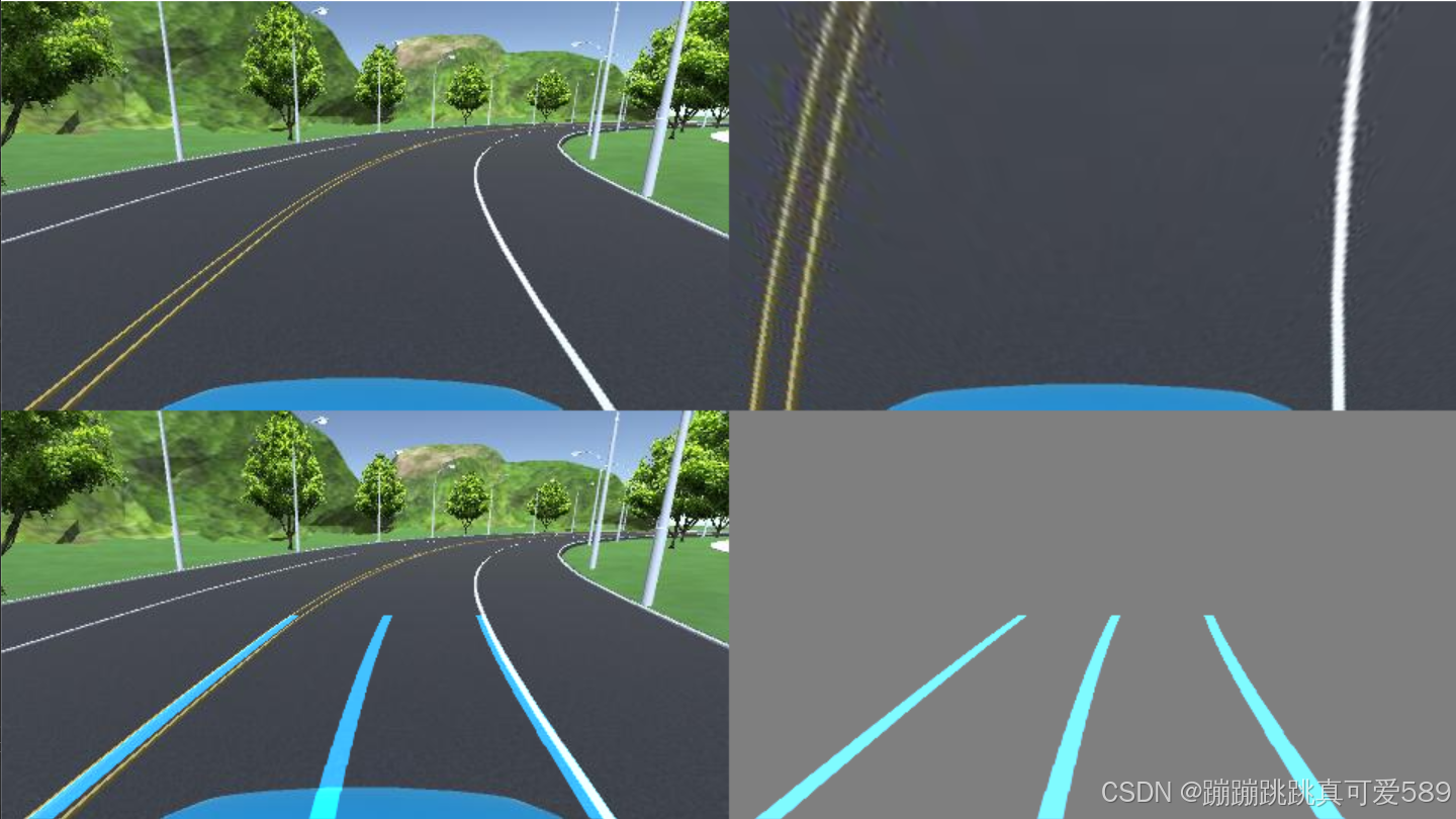
# 将原始图像与透视变换的图像进行水平拼接
concatenate_image1 = np.concatenate((img, img_wrp), axis=1)
# 将加权融合的结果与车道线图像进行水平拼接
concatenate_image2 = np.concatenate((result1, result), axis=1)
# 将两个拼接结果进行垂直拼接,形成最终图像
concatenate_image = np.concatenate((concatenate_image1, concatenate_image2), axis=0)
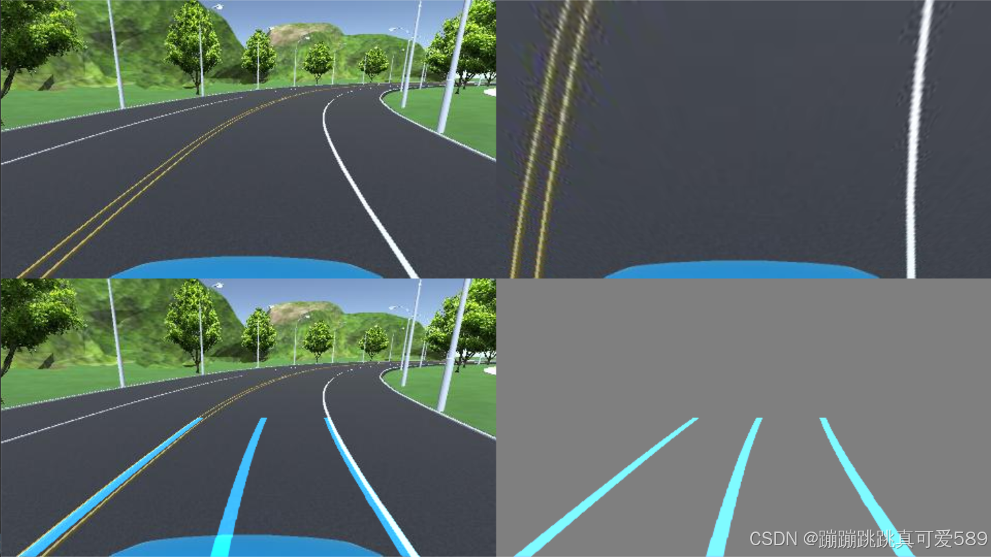
return concatenate_image # 返回最终拼接的图像这段代码的目的是将车道线可视化结果与输入图像进行拼接,以便于展示处理效果。
首先,通过创建一个与 `img_road1` 同样大小的零图像和一个三通道的零图像,准备绘制车道线。
然后,通过将左侧、右侧和中间车道线的坐标点(通过拟合获得)组合在一起以便绘制。
接着,使用 `cv2.polylines` 在零图像上绘制车道线,赋予其颜色和厚度。
接下来,利用逆透视变换将绘制的车道线图像映射到原始图像的空间,并将其与原始图像进行加权融合,生成一个包含车道线的图像。为提供背景对比,创建一个中间灰色的背景图像,并将车道线图像与该背景融合。
随后,将原始图像与透视变换后的图像以及加权融合的结果进行水平拼接。
最终,将这两个拼接结果进行垂直拼接,形成一个展示原始图像、透视图和加权结果的最终图像,便于查看车道线检测与处理效果。该过程为图像处理和计算机视觉任务提供了直观的可视化方式。
五、完整代码
python
import numpy as np
import cv2

# 定义透视变换函数
def img_to_wrp(img):
    height, width,_= img.shape  # 获取输入图像的高度和宽度
    # 定义源点(透视变换前的点)
    src = np.float32(
        [
            [width // 2 - 75, height // 2],  # 左侧车道线的源点
            [width // 2 + 100, height // 2],  # 右侧车道线的源点
            [0, height],  # 底部左侧点
            [width, height]  # 底部右侧点
        ]
    )
    # 定义目标点(透视变换后的点)
    dst = np.float32(
        [
            [0, 0],  # 目标左上角
            [width, 0],  # 目标右上角
            [0, height],  # 目标左下角
            [width, height]  # 目标右下角
        ]
    )
    # 计算透视变换矩阵
    M = cv2.getPerspectiveTransform(src, dst)
    # 计算逆透视变换矩阵
    W = cv2.getPerspectiveTransform(dst, src)
    # 应用透视变换
    img_wrp = cv2.warpPerspective(img, M, (width, height), flags=cv2.INTER_LINEAR)
    return img_wrp, W  # 返回透视变换后的图像和逆变换矩阵

# 定义图像处理函数,提取车道线
def img_road_show1(img):
    img_Gaussian = cv2.GaussianBlur(img, (7, 7), sigmaX=1)  # 对图像进行高斯模糊,减少噪声
    img_gray = cv2.cvtColor(img_Gaussian, cv2.COLOR_BGR2GRAY)  # 将模糊后的图像转换为灰度图像
    img_Sobel = cv2.Sobel(img_gray, -1, dx=1, dy=0)  # 使用Sobel算子进行边缘检测,提取水平边缘
    ret, img_threshold = cv2.threshold(img_Sobel, 127, 255, cv2.THRESH_BINARY)  # 二值化处理

    kernel = np.ones((11, 11), np.uint8)  # 创建一个11x11的结构元素
    img_dilate = cv2.dilate(img_threshold, kernel, iterations=2)  # 膨胀操作,增强白色区域
    img_erode = cv2.erode(img_dilate, kernel, iterations=2)  # 腐蚀操作,去除小噪声
    return img_erode  # 返回处理后的图像


def img_road_show2(img):
    # 将图像从BGR颜色空间转换为HLS颜色空间
    img_hls = cv2.cvtColor(img, cv2.COLOR_BGR2HLS)

    # 提取亮度通道
    l_channel = img_hls[:, :, 1]

    # 将亮度通道进行归一化处理
    l_channel = l_channel / np.max(l_channel) * 255

    # 创建与亮度通道同样大小的零数组
    binary_output1 = np.zeros_like(l_channel)

    # 根据亮度阈值提取车道线区域(亮度值范围为220到255)
    binary_output1[(l_channel > 220) & (l_channel < 255)] = 1

    # 提取黄色车道线
    img_lab = cv2.cvtColor(img, cv2.COLOR_BGR2Lab)  # 将图像转换为Lab颜色空间

    # 将图像的下部分设置为黑色,以减少干扰
    img_lab[:, 240:, :] = (0, 0, 0)

    # 提取Lab颜色空间中的蓝色通道
    lab_b = img_lab[:, :, 2]

    # 如果蓝色通道的最大值大于100则归一化处理
    if np.max(lab_b) > 100:
        lab_b = lab_b / np.max(lab_b) * 255

        # 创建与亮度通道同样大小的零数组
    binary_output2 = np.zeros_like(l_channel)

    # 根据蓝色通道的阈值提取车道线区域(蓝色值范围为212到220)
    binary_output2[(lab_b > 212) & (lab_b < 220)] = 1

    # 创建结构元素,用于形态学操作
    kernel = np.ones((15, 15), np.uint8)

    # 对binary_output2进行膨胀操作,以增强车道线
    binary_output2 = cv2.dilate(binary_output2, kernel, iterations=1)

    # 对膨胀后的图像进行两次腐蚀操作,去除小噪声
    binary_output2 = cv2.erode(binary_output2, kernel, iterations=1)
    binary_output2 = cv2.erode(binary_output2, kernel, iterations=1)

    # 创建一个与binary_output1同样大小的零数组
    binary_output = np.zeros_like(binary_output1)

    # 将两个二值输出结合,提取最终车道线区域
    binary_output[(binary_output1 == 1) | (binary_output2 == 1)] = 1

    # 对最终的二值输出进行膨胀处理
    kernel = np.ones((15, 15), np.uint8)
    img_dilate_binary_output = cv2.dilate(binary_output, kernel, iterations=1)

    # 对膨胀后的图像进行腐蚀处理,以便进一步去噪声
    img_erode_binary_output = cv2.erode(img_dilate_binary_output, kernel, iterations=1)

    # 返回最终处理后的图像
    return img_erode_binary_output


def road_polyfit(img):
    # 获取图像的高度和宽度
    height, width = img.shape
    # 创建一个与输入图像相同大小的RGB图像,用于绘制窗口
    out_img = np.dstack((img, img, img))

    # 计算每一列的白色像素总和,得到直方图
    num_ax0 = np.sum(img, axis=0)

    # 找到直方图左侧和右侧的最高点位置,分别作为车道线的起始点
    img_left_argmax = np.argmax(num_ax0[:width // 2])  # 左侧最高点
    img_right_argmax = np.argmax(num_ax0[width // 2:]) + width // 2  # 右侧最高点

    # 获取图像中所有非零像素的x和y位置
    nonzeroy, nonzerox = np.array(img.nonzero())

    # 定义滑动窗口的数量
    windows_num = 10

    # 定义每个窗口的高度和宽度
    windows_height = height // windows_num
    windows_width = 30

    # 定义在窗口中检测到的白色像素的最小数量
    min_pix = 400

    # 初始化当前窗口的位置,后续会根据检测结果更新
    left_current = img_left_argmax
    right_current = img_right_argmax

    left_pre = left_current  # 记录上一个左侧窗口位置
    right_pre = right_current  # 记录上一个右侧窗口位置

    # 创建空列表以存储左侧和右侧车道线像素的索引
    left_lane_inds = []
    right_lane_inds = []

    # 遍历每个窗口进行车道线检测
    for window in range(windows_num):
        # 计算当前窗口的上边界y坐标
        win_y_high = height - windows_height * (window + 1)
        # 计算当前窗口的下边界y坐标
        win_y_low = height - windows_height * window
        # 计算左侧窗口的左右边界x坐标
        win_x_left_left = left_current - windows_width
        win_x_left_right = left_current + windows_width

        # 计算右侧窗口的左右边界x坐标
        win_x_right_left = right_current - windows_width
        win_x_right_right = right_current + windows_width

        # 在输出图像上绘制当前窗口
        cv2.rectangle(out_img, (win_x_left_left, win_y_high), (win_x_left_right, win_y_low), (0, 255, 0), 2)
        cv2.rectangle(out_img, (win_x_right_left, win_y_high), (win_x_right_right, win_y_low), (0, 255, 0), 2)

        # 找到在当前窗口中符合条件的白色像素索引
        good_left_index = ((nonzeroy >= win_y_high) & (nonzeroy < win_y_low)
                           & (nonzerox >= win_x_left_left) & (nonzerox < win_x_left_right)).nonzero()[0]
        good_right_index = ((nonzeroy >= win_y_high) & (nonzeroy < win_y_low)
                            & (nonzerox >= win_x_right_left) & (nonzerox < win_x_right_right)).nonzero()[0]

        # 将找到的索引添加到列表中
        left_lane_inds.append(good_left_index)
        right_lane_inds.append(good_right_index)

        # 如果找到的左侧像素数量超过阈值,更新左侧窗口位置
        if len(good_left_index) > min_pix:
            left_current = int(np.mean(nonzerox[good_left_index]))
        else:
            # 如果没有找到足够的左侧像素,则根据右侧像素的位置进行偏移
            if len(good_right_index) > min_pix:
                offset = int(np.mean(nonzerox[good_right_index])) - right_pre
                left_current = left_current + offset

                # 如果找到的右侧像素数量超过阈值,更新右侧窗口位置
        if len(good_right_index) > min_pix:
            right_current = int(np.mean(nonzerox[good_right_index]))
        else:
            # 如果没有找到足够的右侧像素,则根据左侧像素的位置进行偏移
            if len(good_left_index) > min_pix:
                offset = int(np.mean(nonzerox[good_left_index])) - left_pre
                right_current = right_current + offset

                # 更新上一个窗口位置
        left_pre = left_current
        right_pre = right_current

        # 将所有的索引连接成一个数组,以便后续提取像素点的坐标
    left_lane_inds = np.concatenate(left_lane_inds)
    right_lane_inds = np.concatenate(right_lane_inds)

    # 提取左侧和右侧车道线像素的位置
    leftx = nonzerox[left_lane_inds]  # 左侧车道线的x坐标
    lefty = nonzeroy[left_lane_inds]  # 左侧车道线的y坐标

    rightx = nonzerox[right_lane_inds]  # 右侧车道线的x坐标
    righty = nonzeroy[right_lane_inds]  # 右侧车道线的y坐标

    # 对左侧和右侧车道线进行多项式拟合,得到拟合曲线的参数
    left_fit = np.polyfit(lefty, leftx, 2)  # 左侧车道线的二次多项式拟合
    right_fit = np.polyfit(righty, rightx, 2)  # 右侧车道线的二次多项式拟合

    # 生成均匀分布的y坐标,用于绘制车道线
    ploty = np.linspace(0, height - 1, height)

    # 根据拟合的多项式计算左侧和右侧车道线的x坐标
    left_fitx = left_fit[0] * ploty ** 2 + left_fit[1] * ploty + left_fit[2]
    right_fitx = right_fit[0] * ploty ** 2 + right_fit[1] * ploty + right_fit[2]

    # 计算中间车道线的位置
    middle_fitx = (left_fitx + right_fitx) // 2

    # 在输出图像上标记车道线像素点
    out_img[lefty, leftx] = [255, 0, 0]  # 左侧车道线
    out_img[righty,rightx]=[0,0,255]# 右侧车道线
    return left_fitx, right_fitx, middle_fitx, ploty


def road_show_concatenate(img, img_wrp, W, img_road1, left_fitx, right_fitx, middle_fitx, ploty):
    # 创建一个与 img_road1 相同大小的零图像,数据类型为 uint8
    wrp_zero = np.zeros_like(img_road1).astype(np.uint8)

    # 创建一个三通道的零图像,用于存放车道线
    color_wrp = np.dstack((wrp_zero, wrp_zero, wrp_zero))

    # 组合车道线点的坐标,用于绘制
    # pts_left, pts_right, pts_middle 是车道线在(y, x)坐标系中的坐标点
    pts_left = np.transpose(np.vstack([left_fitx, ploty]))  # 包括左侧车道线的坐标
    pts_right = np.transpose(np.vstack([right_fitx, ploty]))  # 包括右侧车道线的坐标
    pts_middle = np.transpose(np.vstack([middle_fitx, ploty]))  # 包括中间车道线的坐标

    # 在 zero 图像上绘制车道线
    cv2.polylines(color_wrp, np.int32([pts_left]), isClosed=False, color=(202, 124, 0), thickness=15)  # 绘制左侧车道线
    cv2.polylines(color_wrp, np.int32([pts_right]), isClosed=False, color=(202, 124, 0), thickness=15)  # 绘制右侧车道线
    cv2.polylines(color_wrp, np.int32([pts_middle]), isClosed=False, color=(202, 124, 0), thickness=15)  # 绘制中间车道线

    # 将绘制的车道线通过逆透视变换映射到原始图像的空间
    newwarp = cv2.warpPerspective(color_wrp, W, (img.shape[1], img.shape[0]))

    # 将透视变换后的图像与原始图像进行加权融合
    result1 = cv2.addWeighted(img, 1, newwarp, 1, 0)

    # 创建一个背景图像,并将其初始化为中间灰色
    background_zero = np.zeros_like(img).astype(np.uint8) + 127
    # 将新变换的车道线图像与背景图像进行加权融合
    result = cv2.addWeighted(background_zero, 1, newwarp, 1, 0)

    # 将原始图像与透视变换的图像进行水平拼接
    concatenate_image1 = np.concatenate((img, img_wrp), axis=1)
    # 将加权融合的结果与车道线图像进行水平拼接
    concatenate_image2 = np.concatenate((result1, result), axis=1)
    # 将两个拼接结果进行垂直拼接,形成最终图像
    concatenate_image = np.concatenate((concatenate_image1, concatenate_image2), axis=0)

    return concatenate_image  # 返回最终拼接的图像

if __name__ == '__main__':
    # 读取图像文件 '15.png'
    img = cv2.imread('15.png')

    # 对图像进行透视变换,以便后续的车道线检测
    img_wrp, W = img_to_wrp(img)

    # 通过显示车道线的函数生成一个车道线显示图像
    img_road1 = img_road_show1(img_wrp)

    # 调用 road_polyfit 函数进行车道线的多项式拟合
    # left_fitx, right_fitx, middle_fitx 包含了左右车道线和中间车道线的 x 坐标
    # ploty 包含了 y 坐标的范围
    left_fitx, right_fitx, middle_fitx, ploty = road_polyfit(img_road1)

    # 将处理后的图像与绘制的车道线组合在一起
    concatenate_image = road_show_concatenate(img, img_wrp, W, img_road1, left_fitx, right_fitx, middle_fitx, ploty)

    # 显示最终的拼接图像
    cv2.imshow('concatenate_image', concatenate_image)

    # 等待用户按下任意键,以退出显示窗口
    cv2.waitKey(0)