MATLAB基于统计特征与指数退化模型的风力发电机高速轴承剩余寿命预测

本博客来源于CSDN机器鱼，未同意任何人转载。

更多内容，欢迎点击本专栏目录，查看更多内容。

目录

[0 引言](#0 引言)

[1 数据准备](#1 数据准备)

[1.1 特征提取](#1.1 特征提取)

[1.2 特征数据处理](#1.2 特征数据处理)

[2 RUL模型建立](#2 RUL模型建立)

[2.1 数据集划分](#2.1 数据集划分)

[2.2 特征重要性评估](#2.2 特征重要性评估)

[2.3 退化趋势表征量](#2.3 退化趋势表征量)

[2.4 退化趋势模型搭建](#2.4 退化趋势模型搭建)

References

[3 结语](#3 结语)

---

本博客内容改写自MATLAB2023的案例。首先对数据进行特征提取，然后做特征重要性分析筛选特征，再对特征融合得到表征剩余寿命的退化趋势表征量，最后对表征量进行指数退化建模。

0 引言

很多做故障诊断的学者采用深度学习建模，以故障数据特征为输入，以故障类型做输出。如果训练模型的负载与工况环境与当前我用的机器的负载、工况环境全不一样，这样的模型就没办法迁移到当前机器上做故障诊断。以凯斯西储的滚动轴承数据为例，为了做故障诊断，他们团队人为制造了各种故障类型，并配上不同负载，以此采集数据。那么我自研了一台机器要对其关键轴承做类似的故障诊断，是不是专门把我现在这台机器上的轴承取下来制造不同的故障来采集不同的数据。

显然不是的，这样成本太高了，而且深度学习需要大量的数据来训练，光弄烂一个轴承来采集故障数据是不够的，还需要考虑故障位置、大小、程度、负载等。所以考虑到平台搭建、数据采集成本等问题，我们这篇博客不做轴承的故障诊断了，我们做寿命预测。寿命预测的好处是，我们只需要测量机器全寿命周期的某部件振动参数即可，搭建实验平台的时候也只需要加上电源+电机+轴承+负载+传感器，让电机一直转动，隔几个小时采集一次传感器数据，直到轴承报废。

本示例将展示如何提取表征寿命的特征数据，以及如何构建指数退化模型来实时预测风力涡轮机轴承的剩余使用寿命（RUL）。

1 数据准备

说那么多，其实我也没钱搭建平台，用的还是现有的数据集。

数据集可以在【这里】下载。

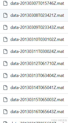
原始数据集采集自一个由20齿小齿轮驱动的2MW风力涡轮机的高速轴，连续采集50天，每天采集6秒的振动信号，连续采集50天，期间出现内圈故障，最终导致轴承失效。

首先可视化数据集：

clc;clear
%% 加载数据
path = 'WindTurbineHighSpeedBearingPrognosis-Data-master';
data = [];

files = dir(fullfile(path, '*.mat')); % 获取所有 .mat 文件的文件信息
fileNames = cell(numel(files),3); % 存储文件名的数组
for i = 1:numel(files)
    name= files(i).name; 
    name = split(name,[".","-"]);
    date = name(2);
    load(fullfile(path,files(i).name));
    fileNames{i,1} = date;% 获取时间
    fileNames{i,2} = vibration; % 获取振动信号
    fileNames{i,3} = tach; % 获取tach转速表
end


%% 可视化
% Sample rate of vibration signal is 97656 Hz. 
fs = 97656; % Hz
tstart = 0;
figure
hold on
for i =1:size(fileNames,1)
    
    v = fileNames{i,2};
    t = tstart + (1:length(v))/fs;
    % Downsample the signal to reduce memory usage
    plot(t(1:10:end), v(1:10:end))
    tstart = t(end);
end
hold off
xlabel('Time (s), 6 second per day, 50 days in total')
ylabel('Acceleration (g)')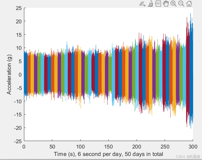

1.1 特征提取

我们从上图可以发现，随着运行时间的增加，振动信号的幅值有着明显的变化，时域中的振动信号显示出信号冲动性的增加趋势，因此可以考虑从时域上提取一部分特征用来表征不同退化程度。主要包括时域信号的均值mean、方差std、偏度skewness、峰度kurtosis、峰峰值peak2peak、均方差rms、峰值因子crestfactor、形状因子shapefactor、脉冲因子ImpulseFactor、边际因子MarginFactor、能量Energy作为时域特征。

此外，频域谱峭度也常用在轴承RUL预测分析中。如下图所示，我们将提取谱峭度中的均值mean、方差std、偏度skewness、峰度kurtosis做为频域特征。

%% 可视化频域谱峭度
colors = parula(50);
figure
hold on
day = 1;
for i =1:size(fileNames,1)
    v = fileNames{i,2};% Get vibration signal and measurement date
    
    % Compute spectral kurtosis with window size = 128
    wc = 128;
    [SK, F] = pkurtosis(v, fs, wc);
    SpectralKurtosis = {table(F, SK)};
    
    % Plot the spectral kurtosis
    plot3(F, day*ones(size(F)), SK, 'Color', colors(day, :))
    fileNames{i,4} = SK; % 保存谱峭度
    % Increment the number of days
    day = day + 1;
end
hold off
xlabel('Frequency (Hz)')
ylabel('Time (day)')
zlabel('Spectral Kurtosis')
grid on
view(-45, 30)
cbar = colorbar;
ylabel(cbar, 'Fault Severity (0 - healthy, 1 - faulty)')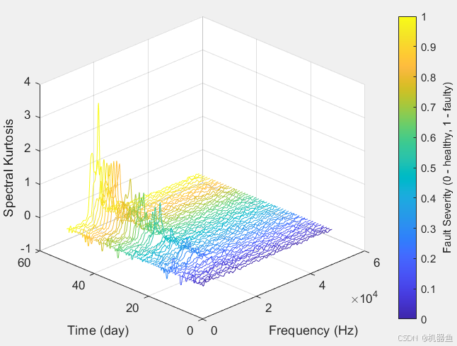

鉴于上述分析，我们写一个循环对时域和频域数据进行特征提取，保存在变量features中，一行为一天的15个特征。

%% 特提提取
features=[];
for i =1:size(fileNames,1)
    v = fileNames{i,2};% 时域信号
    SK = fileNames{i,4};% 频域信号
    % Time Domain Features
    features(i,1) = mean(v);
    features(i,2) = std(v);
    features(i,3) = skewness(v);
    features(i,4) = kurtosis(v);
    features(i,5) = peak2peak(v);
    features(i,6) = rms(v);
    features(i,7) = max(v)/features(i,6);
    features(i,8) = features(i,6)/mean(abs(v));
    features(i,9) = max(v)/mean(abs(v));
    features(i,10) = max(v)/mean(abs(v))^2;
    features(i,11) = sum(v.^2);
    
    % Spectral Kurtosis related features
    features(i,12) = mean(SK);
    features(i,13) = std(SK);
    features(i,14) = skewness(SK);
    features(i,15) = kurtosis(SK);
end
% 取其中两个特征做可视化
figure
subplot(1,2,1)
plot(features(:,2))
ylabel("Std")
xlabel("Day")
subplot(1,2,2)
plot(features(:,12))
ylabel("SK Mean")
xlabel("Day")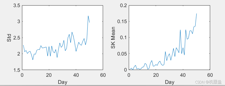

1.2 特征数据处理

由于原始数据存在噪声，对提取的特征应用具有5步滞后窗口的因果移动均值滤波器进行平滑去噪，其中"因果"意味着在移动均值滤波中不使用未来值。

%% 因果移动均值滤波器 去噪 窗口大小5
for i =1:size(features,2)
    featureSmooth(:,i) = movmean(features(:,i), 5);
end
figure

plot(features(:,12))
hold on
plot(featureSmooth(:,12))
ylabel("SK Mean")
legend("原始","去噪")
xlabel("Day")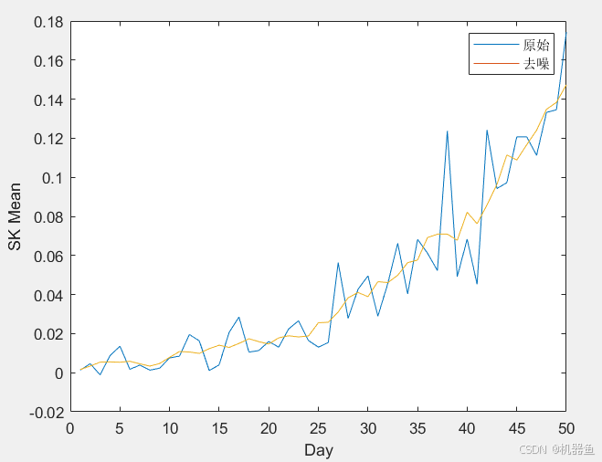

2 RUL模型建立

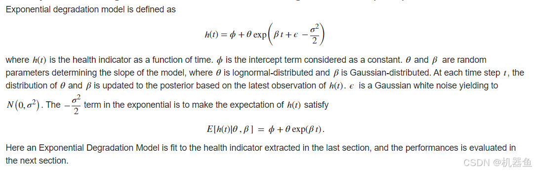
指数退化模型根据其参数先验和最新测量值预测RUL（历史运行故障数据可以帮助估计模型参数先验，但不是必需的）。该模型能够实时检测显著的退化趋势，并在有新的观测结果可用时更新其参数先验。

2.1 数据集划分

在实践中，开发寿命预测算法时无法获得整个生命周期的数据，但可以合理地假设已经收集了生命周期早期的一些数据。因此，我们取生命周期的前20天（40%）收集的数据被视为训练集数据，剩下的为测试集数据。

2.2 特征重要性评估

由于提取的特征是通用的，其中肯定包含不能表征退化趋势的特征，因此首先做重要性分析 ，去掉不重要的特征。我们采用单调性来评估各个特征

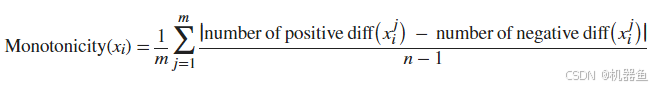
其中n是长度，我们训练集是20天，m代表机器数量，我们只有一台机器的数据，所以m=1；xi是第i种特征，diff(xi)=xi(t)-xi(t-1)；由于我们评估的时候不能包含未来的数据，所以先做的数据集划分，再取训练集的数据做评估，如果直接对featuressmooth，就会包含未来数据的信息，显然是不对的。根据特征重量性图，我们取大于0.15的特征。

%% 特征重要性评估
train_data = featureSmooth(1:20,:);
test_data = featureSmooth(20:end,:);
for i =1:size(train_data,2)
    diffxi=diff(train_data(:,i));
    num_positive=sum(diffxi>0);
    num_negtive=sum(diffxi<0);
    importance(i)=abs(num_positive-num_negtive)/(size(train_data,1)-1);
end
% monotonicity;
figure
bar(importance)
xlabel("特征")
ylabel("单调性")

index = importance>0.15;
train_data=train_data(:,index);
test_data=test_data(:,index);

2.3 退化趋势表征量

提取完不同寿命时的特征量之后该做什么？回到最开始我们的目的：剩余寿命预测，能直接预测吗，预测还有多少天发生故障？这显然是有点困难的，所以我们转变思维，剩余寿命肯定跟某种"行为"有关。打个比方，预测一只坤还能活多久，怎么预测，我们可以通过观众对他跳舞的打分来预测，打分越低表示跳的越差，跳的越差说明他的精力越来越不行了，离噶不远，这里的打分换个名字就是"退化趋势"。那么观众怎么打分，观众是根据这只坤跳舞时，观念其脚跳起的高度、篮球抛起的高度、姿态的舒展程度、坤叫的响亮程度、基你太美的流畅程度等多个因素，通过这些因素的综合评判来进行打分，这些因素我们换个名字就是"特征"。

所以我们还需要根据2.2筛选的特征进行融合，得到"退化趋势"的表征量。这里我们采用主成分分析来搞，代码如下：

%% 特征可视化
meanTrain = mean(train_data);
sdTrain = std(train_data);
trainDataNormalized = (train_data - meanTrain)./sdTrain;
coef = pca(trainDataNormalized);
PCA1 = (featureSelect-meanTrain)./sdTrain * coef(:, 1);
PCA2 =  (featureSelect-meanTrain)./sdTrain* coef(:, 2);

%% PCA可视化
figure
numData = size(featureSelect, 1);
scatter(PCA1, PCA2, [], 1:numData, 'filled')
xlabel('PCA 1')
ylabel('PCA 2')
cbar = colorbar;
ylabel(cbar, ['Time (' day ')'])

figure
subplot(1,2,1)
plot(PCA1, '-o')
xlabel('Time')
ylabel('PCA1')

subplot(1,2,2)
plot(PCA2, '-o')
xlabel('Time')
ylabel('PCA2')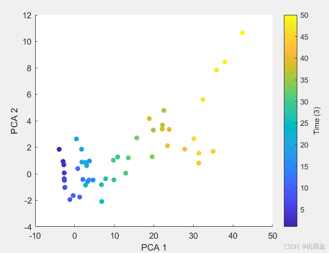

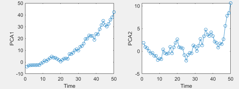
将50天的特征融合，并降至2维，得到PCA1与PCA2，观察可以得出，PCA1具备明显的上升趋势，所以我们可以将PCA1作为退化趋势，即当前的PCA1越大，轴承性能越差，退化越明显，剩余寿命越少。当PCA1达到某个阈值时，我们就认为该轴承已经不能用了。

2.4 退化趋势模型搭建

模型原理如下：

%% 指数衰减RUL估计模型建模
healthIndicator=PCA1;
healthIndicator = healthIndicator - healthIndicator(1);%首先使健康指标从 0 开始。
% 阈值的选择通常基于机器的历史记录或一些特定领域的知识。
% 由于该数据集中没有可用的历史数据，因此选择健康指标的最后一个值作为阈值。
% 建议根据平滑（历史）数据选择阈值，这样可以部分缓解平滑的延迟效应。
threshold = healthIndicator(end);
% 创建一个指数退化模型
mdl = exponentialDegradationModel(...
    'Theta', 1, ...
    'ThetaVariance', 1e6, ...
    'Beta', 1, ...
    'BetaVariance', 1e6, ...
    'Phi', -1, ...
    'NoiseVariance', (0.1*threshold/(threshold + 1))^2, ...
    'SlopeDetectionLevel', 0.05);

% Keep records at each iteration
totalDay = length(healthIndicator) - 1;
estRULs = zeros(totalDay, 1);
trueRULs = zeros(totalDay, 1);
CIRULs = zeros(totalDay, 2);
pdfRULs = cell(totalDay, 1);

% Create figures and axes for plot updating
figure
ax1 = subplot(2, 1, 1);
ax2 = subplot(2, 1, 2);
timeUnit="Day";
for currentDay = 1:totalDay
    
    % Update model parameter posterior distribution
    update(mdl, [currentDay healthIndicator(currentDay)])
    
    % Predict Remaining Useful Life
    [estRUL, CIRUL, pdfRUL] = predictRUL(mdl, ...
                                         [currentDay healthIndicator(currentDay)], ...
                                         threshold);
    trueRUL = totalDay - currentDay + 1;
    
    % Updating RUL distribution plot
    helperPlotTrend(ax1, currentDay, healthIndicator, mdl, threshold, timeUnit);
    helperPlotRUL(ax2, trueRUL, estRUL, CIRUL, pdfRUL, timeUnit)
    
    % Keep prediction results
    estRULs(currentDay) = estRUL;
    trueRULs(currentDay) = trueRUL;
    CIRULs(currentDay, :) = CIRUL;
    pdfRULs{currentDay} = pdfRUL;
    
    % Pause 0.1 seconds to make the animation visible
    pause(0.1)
end

function helperPlotRUL(ax, trueRUL, estRUL, CIRUL, pdfRUL, timeUnit)
    cla(ax)
    hold(ax, 'on')
    plot(ax, pdfRUL{:,1}, pdfRUL{:,2})
    plot(ax, [estRUL estRUL], [0 pdfRUL{find(pdfRUL{:,1} >= estRUL, 1), 2}])
    plot(ax, [trueRUL trueRUL], [0 pdfRUL{find(pdfRUL{:,1} >= trueRUL, 1), 2}], '--')
    idx = pdfRUL{:,1} >= CIRUL(1) & pdfRUL{:,1}<=CIRUL(2);
    area(ax, pdfRUL{idx, 1}, pdfRUL{idx, 2}, ...
        'FaceAlpha', 0.2, 'FaceColor', 'g', 'EdgeColor', 'none');
    hold(ax, 'off')
    ylabel(ax, 'PDF')
    xlabel(ax, ['Time (' timeUnit ')'])
    legend(ax, 'pdf of RUL', 'Estimated RUL', 'True RUL', 'Confidence Interval')
end

function helperPlotTrend(ax, currentDay, healthIndicator, mdl, threshold, timeUnit)

    t = 1:size(healthIndicator, 1);
    HIpred = mdl.Phi + mdl.Theta*exp(mdl.Beta*(t - mdl.InitialLifeTimeValue));
    HIpredCI1 = mdl.Phi + ...
        (mdl.Theta - sqrt(mdl.ThetaVariance)) * ...
        exp((mdl.Beta - sqrt(mdl.BetaVariance))*(t - mdl.InitialLifeTimeValue));
    HIpredCI2 = mdl.Phi + ...
        (mdl.Theta + sqrt(mdl.ThetaVariance)) * ...
        exp((mdl.Beta + sqrt(mdl.BetaVariance))*(t - mdl.InitialLifeTimeValue));
    
    cla(ax)
    hold(ax, 'on')
    plot(ax, t, HIpred)
    plot(ax, [t NaN t], [HIpredCI1 NaN, HIpredCI2], '--')
    plot(ax, t(1:currentDay), healthIndicator(1:currentDay, :))
    plot(ax, t, threshold*ones(1, length(t)), 'r')
    hold(ax, 'off')
    if ~isempty(mdl.SlopeDetectionInstant)
        title(ax, sprintf('Day %d: Degradation detected!\n', currentDay))
    else
        title(ax, sprintf('Day %d: Degradation NOT detected.\n', currentDay))
    end
    ylabel(ax, 'Health Indicator')
    xlabel(ax, ['Time (' timeUnit ')'])
    legend(ax, 'Degradation Model', 'Confidence Interval', ...
        'Health Indicator', 'Threshold', 'Location', 'Northwest')
end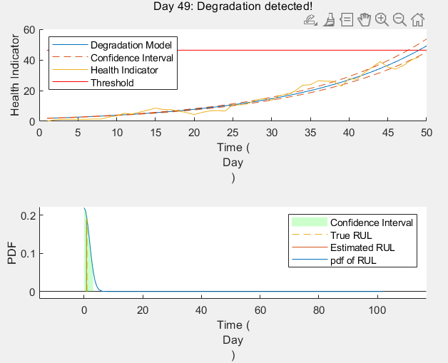

References

1\] Bechhoefer, Eric, Brandon Van Hecke, and David He. "Processing for improved spectral analysis." Annual Conference of the Prognostics and Health Management Society, New Orleans, LA, Oct. 2013. \[2\] Ali, Jaouher Ben, et al. "Online automatic diagnosis of wind turbine bearings progressive degradations under real experimental conditions based on unsupervised machine learning." Applied Acoustics 132 (2018): 167-181. \[3\] Saidi, Lotfi, et al. "Wind turbine high-speed shaft bearings health prognosis through a spectral Kurtosis-derived indices and SVR." Applied Acoustics 120 (2017): 1-8. \[4\] Coble, Jamie Baalis. "Merging data sources to predict remaining useful life--an automated method to identify prognostic parameters." (2010). \[5\] Saxena, Abhinav, et al. "Metrics for offline evaluation of prognostic performance." International Journal of Prognostics and Health Management 1.1 (2010): 4-23. ## 3 结语 更多内容请点击【[专栏](https://blog.csdn.net/qq_41043389/article/details/146406985 "专栏")】获取。您的点赞是我更新MATLAB1000个案例分析的动力。