PINN：用深度学习PyTorch求解微分方程

神经网络技术已在计算机视觉与自然语言处理等多个领域实现了突破性进展。然而在微分方程求解领域，传统神经网络因其依赖大规模标记数据集的特性而表现出明显局限性。物理信息神经网络(Physics-Informed Neural Networks, PINN)通过将物理定律直接整合到学习过程中，有效弥补了这一不足，使其成为求解常微分方程(ODE)和偏微分方程(PDE)的高效工具。

传统神经网络模型需要依赖规模庞大的标记数据集，而这类数据的采集往往成本高昂且耗时显著。PINN通过将物理定律（具体表现为微分方程）融入训练过程，显著提高了数据利用效率。这种方法使得在流体动力学、量子力学和气候系统建模等科学领域实现基于数据的科学发现成为可能，为跨学科研究提供了新的技术路径。

求解微分方程一般方法

有如下微分方程：

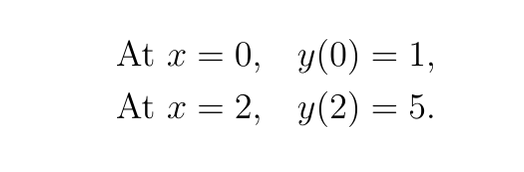
边界条件

由于

对 x 积分一次可得

再次积分，我们得到

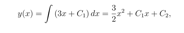
现在，应用边界条件：

1. 对于 y(0)=1

1. 对于 y(2)=5：

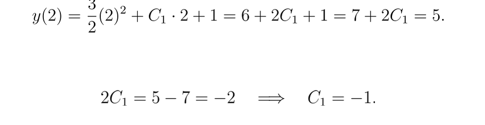
因此，解析解为：

用神经网络解决微分方程

该方法称为 PINN（物理信息神经网络），在我们的示例中的工作方式如下：

神经网络近似：

• 我们定义一个神经网络 y(θ,x)，其中 θ 表示网络参数（权重和偏差）。该网络旨在近似微分方程的解 y(x)。

• 在我们的例子中，神经网络是一个小型全连接网络（具有一个或多个隐藏层），它以空间坐标 x 作为输入并输出 y(x) 的近似值。

自动微分：

• 在这种情况下使用神经网络的一个主要好处是大多数现代深度学习库（如 PyTorch）都支持自动区分。

• 这意味着我们可以直接从网络输出计算关于输入 x 的导数 y′(x) 和 y′′(x)。

残差计算：

• 对于 ODE

我们将残差 r(x) 定义为：

在网络近似精确的点处，残差应该为零。

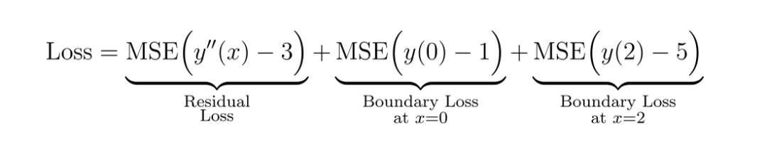
损失函数：

• PINN 方法中的损失函数由两部分组成：

• 残差损失：在域内的一组内部搭配点处计算残差 r(x) 的均方误差 (MSE)。该项强制网络的预测满足微分方程。

• 边界条件损失：网络预测与给定边界条件之间的差异的 MSE。

  

• 总损失为：

PINN的技术特性与创新点

PINN与传统神经网络的根本区别在于，它不依赖于标记数据集进行学习，而是将微分方程约束直接嵌入到损失函数中。这意味着模型学习得到的函数*yNN(x)*需同时满足：

• 给定的微分方程约束条件

• 特定的边界条件和初始条件

PINN框架中的偏微分方程(PDE)通常表示为：

其中

以二阶微分方程为例：

这表明所求函数y(x)必须严格满足该方程。

基于PINN求解微分方程的实践案例

步骤1： 导入必要的库函数

import torch
import torch.nn as nn
import torch.optim as optim
import matplotlib.pyplot as plt
import numpy as np

步骤2： 定义 y(x) 的神经网络近似值

class ODE_Net(nn.Module):
    def __init__(self, hidden_units=20):
        super(ODE_Net, self).__init__()
        self.layer1 = nn.Linear(1, hidden_units)
        self.layer2 = nn.Linear(hidden_units, hidden_units)
        self.layer3 = nn.Linear(hidden_units, 1)
        self.activation = nn.Tanh()
        
    def forward(self, x):
        out = self.activation(self.layer1(x))
        out = self.activation(self.layer2(out))
        out = self.layer3(out)
        return out

步骤3：计算 ODE 残差

def residual(model, x):
    """
    Compute the ODE residual:
        y''(x) - 3 = 0.
    """
    # Enable gradients for x
    x.requires_grad_(True)
    y = model(x)
    
    # Compute first derivative: y'(x)
    dydx = torch.autograd.grad(
        y, x,
        grad_outputs=torch.ones_like(y),
        create_graph=True
    )[0]
    
    # Compute second derivative: y''(x)
    d2ydx2 = torch.autograd.grad(
        dydx, x,
        grad_outputs=torch.ones_like(dydx),
        create_graph=True
    )[0]
    
    # Compute the residual of the ODE: y''(x) - 3
    res = d2ydx2 - 3.0
    return res

步骤4：损失函数

def boundary_loss(model):
    """
    Compute the loss associated with the boundary conditions:
    y(0)=1 and y(2)=5.
    """
    # Boundary condition at x=0: y(0)=1
    x0 = torch.tensor([[0.0]], device=device, requires_grad=True)
    y0 = model(x0)
    loss_bc0 = (y0 - 1.0)**2
    
    # Boundary condition at x=2: y(2)=5
    x2 = torch.tensor([[2.0]], device=device, requires_grad=True)
    y2 = model(x2)
    loss_bc2 = (y2 - 5.0)**2
    
    return loss_bc0 + loss_bc2

步骤5：模型训练

  # Initialize the model and optimizer
  model = ODE_Net(hidden_units=20).to(device)
  optimizer = optim.Adam(model.parameters(), lr=1e-3)
  num_epochs = 5000

# Generate interior points in the domain [0,2]
  N_interior = 50
  x_interior = 2 * torch.rand(N_interior, 1, device=device)  # uniformly distributed in [0,2]

# Training loop
for epoch in range(num_epochs):
      model.train()
      optimizer.zero_grad()
      
      # Compute the residual loss at interior points
      r_interior = residual(model, x_interior)
      loss_res = torch.mean(r_interior**2)
      
      # Compute the boundary condition loss
      loss_bc = boundary_loss(model)
      
      # Total loss is the sum of the residual and boundary losses
      loss = loss_res + loss_bc
      loss.backward()
      optimizer.step()
      
      if epoch % 500 == 0:
          print(f"Epoch {epoch}, Loss: {loss.item():.6e}")

# Evaluate and compare the solution
  model.eval()
  x_test = torch.linspace(0, 2, 100, device=device).unsqueeze(1)
  y_pred = model(x_test).detach().cpu().numpy().flatten()
  x_test_np = x_test.cpu().numpy().flatten()

  
Epoch 0, Loss: 3.222174e+01
Epoch 500, Loss: 1.378794e-01
Epoch 1000, Loss: 5.264541e-03
Epoch 1500, Loss: 3.903809e-03
Epoch 2000, Loss: 3.040434e-03
Epoch 2500, Loss: 2.319159e-03
Epoch 3000, Loss: 1.656389e-03
Epoch 3500, Loss: 9.695904e-04
Epoch 4000, Loss: 4.545122e-04
Epoch 4500, Loss: 2.485181e-04

步骤6：对比精确度

  # Analytical solution: y(x) = (3/2)x^2 - x + 1
  y_true = 1.5 * x_test_np**2 - x_test_np + 1
    
  plt.figure(figsize=(8, 4))
  plt.plot(x_test_np, y_pred, label="PINN Solution")
  plt.plot(x_test_np, y_true, '--', label="Analytical Solution")
  plt.xlabel("x")
  plt.ylabel("y(x)")
  plt.legend()
  plt.title("ODE: y''(x) - 3 = 0 with y(0)=1, y(2)=5")
  plt.show()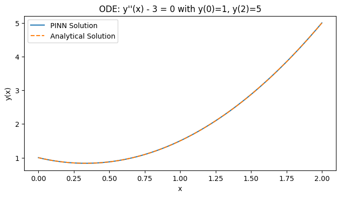

使用 PINN 求解更复杂的 ODE

class ODE_Net(nn.Module):
    def __init__(self, hidden_units=20):
        super(ODE_Net, self).__init__()
        self.layer1 = nn.Linear(1, hidden_units)
        self.layer2 = nn.Linear(hidden_units, hidden_units)
        self.layer3 = nn.Linear(hidden_units, hidden_units)
        self.layer4 = nn.Linear(hidden_units, 1)
        self.activation = nn.Tanh()

    def forward(self, x):
        out = self.activation(self.layer1(x))
        out = self.activation(self.layer2(out))
        out = self.activation(self.layer3(out))
        out = self.layer4(out)
        return out

def residual(model, x):
    x.requires_grad_(True)
    y = model(x)
    y_x = torch.autograd.grad(y, x, grad_outputs=torch.ones_like(y),
                                create_graph=True)[0]
    y_xx = torch.autograd.grad(y_x, x, grad_outputs=torch.ones_like(y_x),
                                 create_graph=True)[0]
    y_xxx = torch.autograd.grad(y_xx, x, grad_outputs=torch.ones_like(y_xx),
                                  create_graph=True)[0]
    y_xxxx = torch.autograd.grad(y_xxx, x, grad_outputs=torch.ones_like(y_xxx),
                                   create_graph=True)[0]    
    res = y_xxxx - 2*y_xxx + y_xx
    return res

def boundary_loss(model):
    x0 = torch.tensor([[0.0]], device=device, requires_grad=True)
    y0 = model(x0)
    
    y0_x = torch.autograd.grad(y0, x0, grad_outputs=torch.ones_like(y0),
                                 create_graph=True)[0]
    y0_xx = torch.autograd.grad(y0_x, x0, grad_outputs=torch.ones_like(y0_x),
                                  create_graph=True)[0]
    y0_xxx = torch.autograd.grad(y0_xx, x0, grad_outputs=torch.ones_like(y0_xx),
                                   create_graph=True)[0]
    
    bc1 = y0 - 1.0      # y(0) = 1
    bc2 = y0_x - 0.0    # y'(0) = 0
    bc3 = y0_xx - (-1.0)  # y''(0) = -1  -> y0_xx + 1 = 0
    bc4 = y0_xxx - 2.0# y'''(0) = 2
    
    loss_bc = bc1**2 + bc2**2 + bc3**2 + bc4**2
    return loss_bc

def main():
    model = ODE_Net(hidden_units=20).to(device)
    optimizer = optim.Adam(model.parameters(), lr=1e-3)
    num_epochs = 10000
    
    N_interior = 50
    x_interior = torch.rand(N_interior, 1, device=device)
    
    for epoch in range(num_epochs):
        model.train()
        optimizer.zero_grad()
        
        r_interior = residual(model, x_interior)
        loss_res = torch.mean(r_interior**2)
        
        loss_bc = boundary_loss(model)        
        loss = loss_res + loss_bc
        loss.backward()
        optimizer.step()
        
        if epoch % 500 == 0:
            print(f"Epoch {epoch}, Loss: {loss.item():.6e}")
    
    model.eval()
    x_test = torch.linspace(0, 1, 100, device=device).unsqueeze(1)
    y_pred = model(x_test).detach().cpu().numpy().flatten()
    x_test_np = x_test.cpu().numpy().flatten()
    
    # Analytical solution: y(x) = 8 + 4x - 7e^x + 3xe^x
    y_true = 8 + 4*x_test_np - 7*np.exp(x_test_np) + 3*x_test_np*np.exp(x_test_np)
    
    plt.figure(figsize=(8,4))
    plt.plot(x_test_np, y_pred, label="Solution using PINN")
    plt.plot(x_test_np, y_true, '--', label="Analytical solution")
    plt.xlabel("x")
    plt.ylabel("y(x)")
    plt.legend()
    plt.show()

if __name__ == "__main__":
    main()

Epoch 0, Loss: 6.779857e+00
Epoch 500, Loss: 2.092192e-01
Epoch 1000, Loss: 4.828146e-02
Epoch 1500, Loss: 3.233620e-02
Epoch 2000, Loss: 3.518355e-04
Epoch 2500, Loss: 2.392017e-04
Epoch 3000, Loss: 1.745588e-04
Epoch 3500, Loss: 1.332138e-04
Epoch 4000, Loss: 1.039377e-04
Epoch 4500, Loss: 3.754102e-03
Epoch 5000, Loss: 7.414911e-05
Epoch 5500, Loss: 5.272599e-05
Epoch 6000, Loss: 4.189969e-05
Epoch 6500, Loss: 1.759992e-03
Epoch 7000, Loss: 1.593289e-04
Epoch 7500, Loss: 2.400937e-05
Epoch 8000, Loss: 8.885263e-03
Epoch 8500, Loss: 6.434955e-05
Epoch 9000, Loss: 1.761451e-05
Epoch 9500, Loss: 1.477061e-05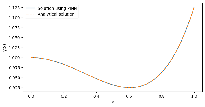

通过结果可以看出，我们已经成功地使用PINN方法求解了上述微分方程，并获得了与解析解高度一致的数值解。

写在最后

物理信息神经网络(PINN)代表了一种在微分方程求解领域的重要技术突破，它将深度学习与物理定律有机结合，为传统数值求解方法提供了一种高效、数据驱动的替代方案。PINN方法不仅在理论上具有创新性，同时在实际应用中展现出广阔的应用前景，为复杂物理系统的建模与分析提供了新的研究路径。