Logistic Regression(逻辑回归)是一种用于处理二分类问题的统计学习方法。它基于线性回归 模型,通过Sigmoid函数将输出映射到0, 1范围内,表示概率。逻辑回归常被用于预测某个实 例属于正类别的概率。
一、数据集介绍

在本例中,使用了乳腺癌数据集 Breast Cancer - UCI Machine Learning Repository,其中包含 关于病人的信息,目标是预测肿瘤是否为无复发事件(no-recurrence-events)或有复发事件 (recurrence-events)。
数据集地址
| Variable Name | Role | Type | Demographic | Description | Units | Missing Values |
|---|---|---|---|---|---|---|
| Class | Target | Binary | no-recurrence-events, recurrence-events | no | ||
| age | Feature | Categorical | Age | 10-19, 20-29, 30-39, 40-49, 50-59, 60-69, 70-79, 80-89, 90-99 | years | no |
| menopause | Feature | Categorical | lt40, ge40, premeno | no | ||
| tumor-size | Feature | Categorical | 0-4, 5-9, 10-14, 15-19, 20-24, 25-29, 30-34, 35-39, 40-44, 45-49, 50-54, 55-59 | no | ||
| inv-nodes | Feature | Categorical | 0-2, 3-5, 6-8, 9-11, 12-14, 15-17, 18-20, 21-23, 24-26, 27-29, 30-32, 33-35, 36-39 | no | ||
| node-caps | Feature | Binary | yes, no | yes | ||
| deg-malig | Feature | Integer | 1, 2, 3 | no | ||
| breast | Feature | Binary | left, right | no | ||
| breast-quad | Feature | Categorical | left-up, left-low, right-up, right-low, central | yes | ||
| irradiat | Feature | Binary | yes, no | no |
其他变量信息
类:no-recurrence-events、recurrence-events
年龄:10-19、20-29、30-39、40-49、50-59、60-69、70-79、80-89、90-99。
更年期:LT40、GE40、Premeno。
肿瘤大小:0-4、5-9、10-14、15-19、20-24、25-29、30-34、35-39、40-44、45-49、50-54、55-59。
INV 节点:0-2、3-5、6-8、9-11、12-14、15-17、18-20、21-23、24-26、27-29、30-32、33-35、36-39。
node-caps:是的,不是。
度-马利格: 1, 2, 3.
胸部:左、右。
乳房四头肌:左上、左低、右上、右低、中央。
Irradiat:是的,不是。
二、设计思路
2.1、读取数据
python
import pandas as pd
names = ['Class', 'age', 'menopause', 'tumor-size', 'inv-nodes', 'node-caps', 'deg-malig', 'breast', 'breast-quad', 'irradiat']
df=pd.read_table('breast-cancer.data',names=names,sep=',')
2.2、数据清洗
python
import numpy as np
df=df.replace('?',np.nan)
df.dropna(axis=0,inplace=True)
2.3、划分特征
python
X=df.drop(columns=['Class'],axis=1)
y=df['Class']
2.4、one-hot独热编码
python
X=pd.get_dummies(X)2.5、划分训练集和测试集
python
from sklearn.model_selection import train_test_split
X_train,X_test,y_train,y_test=train_test_split(X,y,train_size=0.8,random_state=42)
2.6、标准化
python
from sklearn.preprocessing import StandardScaler
scaler=StandardScaler()
X_train_scaler=scaler.fit_transform(X_train)
X_test_scaler=scaler.transform(X_test)
2.7、特征标签
python
from sklearn.preprocessing import LabelEncoder
labelencoder=LabelEncoder()
y_train_labelencoder=labelencoder.fit_transform(y_train)
y_test_labelencoder=labelencoder.transform(y_test)
2.8、加载逻辑回归模型拟合
python
from sklearn.linear_model import LogisticRegression
lr=LogisticRegression(C=1e5)
lr.fit(X_train_scaler,y_train_labelencoder)
2.9、模型评估
python
from sklearn.metrics import roc_curve,auc

prepro = lr.predict_proba(X_test_scaler)[:, 1]
fpr, tpr, thresholds = roc_curve(y_test_labelencoder, prepro)
roc_auc=auc(fpr,tpr)
2.10、可视化
python
from matplotlib import pylab as plt
plt.figure(figsize=(10, 6))
plt.plot(fpr, tpr, color='darkorange', lw=2, label=f'AUC = {roc_auc:.2f}')
plt.plot([0, 1], [0, 1], color='navy', lw=2, linestyle='--')
plt.xlabel('False Positive Rate')
plt.ylabel('True Positive Rate')
plt.title('Receiver Operating Characteristic (ROC) Curve')
plt.legend(loc='lower right')
plt.show()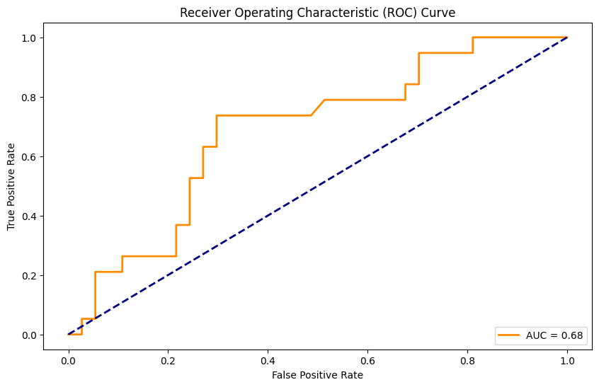
三、完整代码
python
import pandas as pd
from sklearn.preprocessing import StandardScaler
from sklearn.model_selection import train_test_split
from sklearn.preprocessing import LabelEncoder
import numpy as np
from sklearn.metrics import roc_curve, auc
from sklearn.linear_model import LogisticRegression
from matplotlib import pylab as plt

# 定义数据集的列名称
names = ['Class', 'age', 'menopause', 'tumor-size', 'inv-nodes', 'node-caps', 'deg-malig', 'breast', 'breast-quad', 'irradiat']

# 读取数据集,并将第一行作为列名
df = pd.read_table('breast-cancer.data', names=names, sep=',')

# 替换缺失值的标记'?'为NaN,并删除含有缺失值的行
df = df.replace('?', np.nan)
df.dropna(axis=0, inplace=True)

# 分离特征和目标变量
X = df.drop(columns=['Class'], axis=1)  # 特征数据
y = df['Class']  # 目标变量

# 将分类特征进行独热编码
X = pd.get_dummies(X)

# 划分训练集和测试集,训练集占80%
X_train, X_test, y_train, y_test = train_test_split(X, y, train_size=0.8, random_state=42)

# 数据标准化
scaler = StandardScaler()
X_train_scaler = scaler.fit_transform(X_train)  # 对训练数据进行标准化
X_test_scaler = scaler.transform(X_test)        # 对测试数据进行同样的标准化

# 标签编码
labelencoder = LabelEncoder()
y_train_labelencoder = labelencoder.fit_transform(y_train)  # 将训练标签编码为0/1
y_test_labelencoder = labelencoder.transform(y_test)        # 将测试标签编码为0/1

# 实例化逻辑回归模型,正则化参数C设置为1e5
lr = LogisticRegression(C=1e5)
lr.fit(X_train_scaler, y_train_labelencoder)  # 训练模型

# 预测测试集中每个样本属于正类的概率
prepro = lr.predict_proba(X_test_scaler)[:, 1]
# 计算ROC曲线
fpr, tpr, thresholds = roc_curve(y_test_labelencoder, prepro)
roc_auc = auc(fpr, tpr)  # 计算AUC值

# 绘制ROC曲线
plt.figure(figsize=(10, 6))
plt.plot(fpr, tpr, color='darkorange', lw=2, label=f'AUC = {roc_auc:.2f}')  # 绘制ROC曲线
plt.plot([0, 1], [0, 1], color='navy', lw=2, linestyle='--')  # 绘制随机猜测的对角线
plt.xlabel('假阳率 (False Positive Rate)')  # X轴标签
plt.ylabel('真阳率 (True Positive Rate)')  # Y轴标签
plt.title('接收者操作特征 (ROC) 曲线')  # 图表标题
plt.legend(loc='lower right')  # 图例位置
plt.show()  # 显示图表
设计思路
-
数据读取和预处理:
加载数据: 使用
pd.read_table函数读取乳腺癌数据集,指定数据分隔符为逗号,并为每列定义合适的列名,增加可读性。处理缺失值: 数据中的缺失值用"?"表示,将其替换为NaN,并使用dropna方法删除所有包含缺失值的行,确保后续分析和建模的数据质量。 -
特征和标签的分离:
分离特征与标签: 将数据集拆分为特征(
X)和目标变量(y),其中X为特征数据,y为类别标签(如"良性"或"恶性")。 -
类别特征的处理:
独热编码: 使用
pd.get_dummies将分类特征转换为数值型特征,生成更易于模型处理的二进制特征矩阵。独热编码将每个类别值转化为可互斥的二进制值,从而使得模型能够理解分类数据。 -
数据集划分:
训练集与测试集划分: 使用
train_test_split按照80%的比例将数据集分为训练集和测试集,以保障模型训练和验证的有效性。这种方法使得模型能够在独立的数据上进行测试,从而避免过拟合。 -
标准化处理:
数据标准化: 利用
StandardScaler对特征数据进行标准化,使其均值为0,方差为1。这一步骤可以消除特征之间由于量纲不同而带来的影响,从而提高模型的收敛速度和稳定性。 -
标签编码:
编码目标变量: 采用
LabelEncoder对目标变量进行编码,将标签(如"良性"、"恶性")转换为0和1的数值形式,以便于后续模型的训练。 -
模型训练:
实例化逻辑回归模型: 采用
LogisticRegression类,设置正则化参数C(此处设定为1e5)来控制模型的复杂度。模型训练: 使用标准化后的训练数据对模型进行拟合(fit),建立分类模型。 -
性能评估:
概率预测: 在测试集上使用训练好的逻辑回归模型进行概率预测,通过
predict_proba函数获取分类为正类的概率。计算ROC曲线: 使用roc_curve函数计算真正率(TPR)和假正率(FPR),以评估模型在不同阈值下的性能。计算AUC值: 利用auc函数计算曲线下的面积(Area Under Curve,AUC),作为量化模型性能的指标。 -
可视化效果:
绘制ROC曲线: 使用Matplotlib库绘制ROC曲线,通过可视化手段展示模型在分类任务中的表现,同时标注AUC值以便于理解模型的好坏。图例、标签和标题增强了图表的可读性。