R4打卡——tensorflow实现火灾预测

🍨 本文为 🔗365天深度学习训练营中的学习记录博客

• 🍖 原作者： K同学啊

1.检查GPU

import tensorflow as tf
import pandas     as pd
import numpy      as np

gpus = tf.config.list_physical_devices("GPU")
if gpus:
    tf.config.experimental.set_memory_growth(gpus[0], True)  #设置GPU显存用量按需使用
    tf.config.set_visible_devices([gpus[0]],"GPU")
print(gpus)

​

2.查看数据

import pandas as pd
import numpy as np

df_1 = pd.read_csv("data/woodpine2.csv")
df_1

import matplotlib.pyplot as plt
import seaborn as sns

plt.rcParams['savefig.dpi'] = 500 #图片像素
plt.rcParams['figure.dpi']  = 500 #分辨率

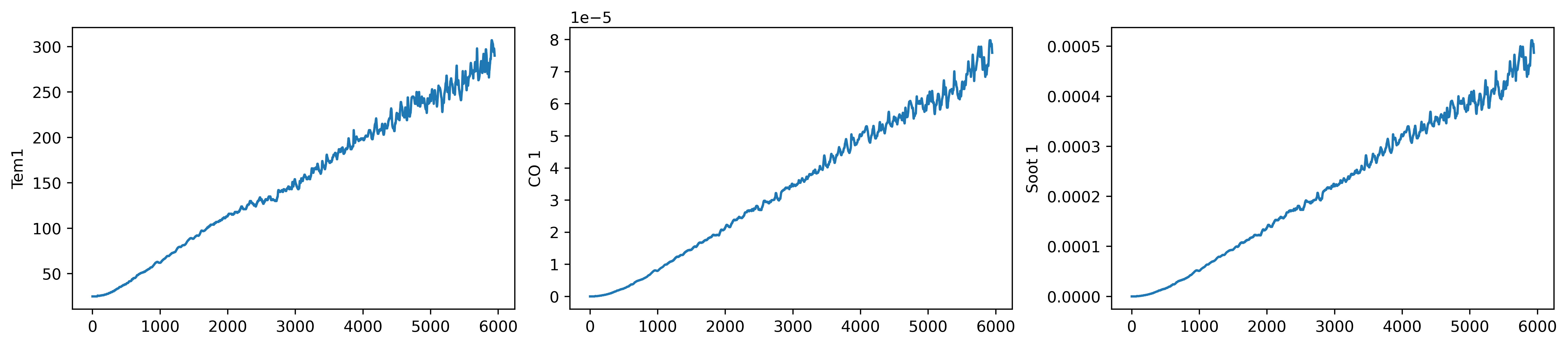
fig, ax =plt.subplots(1,3,constrained_layout=True, figsize=(14, 3))

sns.lineplot(data=df_1["Tem1"], ax=ax[0])
sns.lineplot(data=df_1["CO 1"], ax=ax[1])
sns.lineplot(data=df_1["Soot 1"], ax=ax[2])
plt.show()

dataFrame = df_1.iloc[:,1:]
dataFrame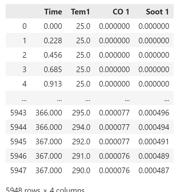

​​

​

3.划分数据集

width_X = 8
width_y = 1

X = []
y = []

in_start = 0

for _, _ in df_1.iterrows():
    in_end  = in_start + width_X
    out_end = in_end   + width_y
    
    if out_end < len(dataFrame):
        X_ = np.array(dataFrame.iloc[in_start:in_end , ])
        X_ = X_.reshape((len(X_)*3))
        y_ = np.array(dataFrame.iloc[in_end  :out_end, 0])

        X.append(X_)
        y.append(y_)
    
    in_start += 1

X = np.array(X)
y = np.array(y)

X.shape, y.shape

from sklearn.preprocessing import MinMaxScaler

#将数据归一化，范围是0到1
sc       = MinMaxScaler(feature_range=(0, 1))
X_scaled = sc.fit_transform(X)
X_scaled.shape

X_scaled = X_scaled.reshape(len(X_scaled),width_X,3)
X_scaled.shape

X_train = np.array(X_scaled[:5000]).astype('float64')
y_train = np.array(y[:5000]).astype('float64')

X_test  = np.array(X_scaled[5000:]).astype('float64')
y_test  = np.array(y[5000:]).astype('float64')

X_train.shape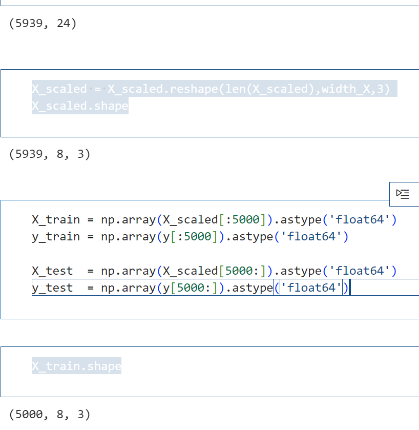

​​​​

​​​​​

4.创建模型

from tensorflow.keras.models import Sequential
from tensorflow.keras.layers import Dense,LSTM,Bidirectional
from tensorflow.keras        import Input

# 多层 LSTM
model_lstm = Sequential()
model_lstm.add(LSTM(units=64, activation='relu', return_sequences=True,
               input_shape=(X_train.shape[1], 3)))
model_lstm.add(LSTM(units=64, activation='relu'))

model_lstm.add(Dense(width_y))

​

​​​​5.编译及训练模型

# 只观测loss数值，不观测准确率，所以删去metrics选项
model_lstm.compile(optimizer=tf.keras.optimizers.Adam(1e-3),
                   loss='mean_squared_error')  # 损失函数用均方误差

history_lstm = model_lstm.fit(X_train, y_train, 
                         batch_size=64, 
                         epochs=40, 
                         validation_data=(X_test, y_test),
                         validation_freq=1)

​

​

​​​​​

6.结果可视化

# 支持中文
plt.rcParams['font.sans-serif'] = ['SimHei']  # 用来正常显示中文标签
plt.rcParams['axes.unicode_minus'] = False  # 用来正常显示负号

plt.figure(figsize=(5, 3),dpi=120)

plt.plot(history_lstm.history['loss']    , label='LSTM Training Loss')
plt.plot(history_lstm.history['val_loss'], label='LSTM Validation Loss')

plt.title('Training and Validation Loss')
plt.legend()
plt.show()

predicted_y_lstm = model_lstm.predict(X_test)                        # 测试集输入模型进行预测

y_test_one = [i[0] for i in y_test]
predicted_y_lstm_one = [i[0] for i in predicted_y_lstm]

plt.figure(figsize=(5, 3),dpi=120)
# 画出真实数据和预测数据的对比曲线
plt.plot(y_test_one[:1000], color='red', label='真实值')
plt.plot(predicted_y_lstm_one[:1000], color='blue', label='预测值')

plt.title('Title')
plt.xlabel('X')
plt.ylabel('Y')
plt.legend()
plt.show()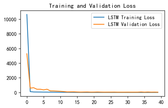

​​​​​

​​​​​7.模型评估

from sklearn import metrics
"""
RMSE ：均方根误差  ----->  对均方误差开方
R2   ：决定系数，可以简单理解为反映模型拟合优度的重要的统计量
"""
RMSE_lstm  = metrics.mean_squared_error(predicted_y_lstm, y_test)**0.5
R2_lstm    = metrics.r2_score(predicted_y_lstm, y_test)

print('均方根误差: %.5f' % RMSE_lstm)
print('R2: %.5f' % R2_lstm)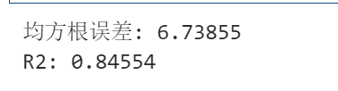

​​​​​​​​​​​​​

总结：

1. 背景与目标

通过使用 TensorFlow 框架构建了一个基于 LSTM 的时间序列预测模型。任务是从给定的数据集中提取特征（Tem1, CO 1, Soot 1），并利用前8个时间段的数据预测第9个时间段的目标变量（Tem1）。整个流程包括数据预处理、模型构建、训练、评估和结果可视化等关键步骤。

---

2. 代码流程概述

（1）检查GPU

• 使用 tf.config.list_physical_devices("GPU") 检查是否有可用的 GPU 资源。
• 设置 GPU 显存按需分配，避免显存不足的问题。
• GPU 加速可以显著提升模型训练效率，特别是在处理大规模数据时。

（2）查看数据

• 数据集包含三列：Tem1（目标变量）、CO 1 和 Soot 1。
• 使用 seaborn 和 matplotlib 对数据进行可视化，观察各特征的时间序列趋势。
• 数据预处理包括归一化操作，将所有特征值缩放到 [0, 1] 范围内，以便模型更好地收敛。

（3）划分数据集

• 将数据划分为输入特征 X 和目标变量 y：
  • 输入 X 包含连续的8个时间步的特征值，并将其展平为 (len(X)*3) 的形式。
  • 输出 y 是第9个时间步的目标值。
• 数据集进一步划分为训练集和测试集，并转化为 NumPy 数组格式，方便后续模型训练。
• 归一化后的数据被重新调整为适合 LSTM 输入的形状 (样本数, 时间步数, 特征数)。

（4）创建模型

• 定义了一个两层 LSTM 网络模型：
  • 第一层 LSTM 的隐藏单元数为64，激活函数为 ReLU，并返回序列以供下一层使用。
  • 第二层 LSTM 进一步提取时间序列特征。
  • 最后通过全连接层输出单个预测值。
• 模型的设计考虑了时间序列数据的特点，能够捕捉长期依赖关系。

（5）编译与训练模型

• 使用均方误差（MSE）作为损失函数，Adam 优化器作为优化算法。
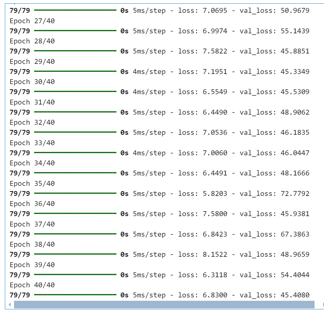
• 训练过程中，设置了批量大小为64，训练40个 epoch，并在每个 epoch 后验证模型性能。
• 验证频率设置为1，确保每次训练后都能看到验证集上的表现。

（6）结果可视化

• 绘制了训练集和测试集的损失曲线，直观地展示了模型的收敛情况。
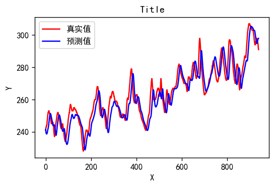
• 对比了真实值与预测值的时间序列曲线，验证了模型的预测能力。
• 使用列表推导式将预测值和真实值压缩为一维数组，便于绘图。

（7）模型评估

• 使用均方根误差（RMSE）和决定系数（R²）评估模型性能：
  • RMSE 衡量预测值与真实值之间的偏差。
  • R² 反映模型对数据变化的拟合程度。
• 结果表明，模型在测试集上具有一定的预测能力，但仍存在改进空间。

---

3. 代码亮点

• 数据预处理：通过归一化处理和滑动窗口方法，有效地构造了适合LSTM模型的输入数据。
• 模型设计：采用了双层LSTM结构，能够更好地捕捉时间序列中的复杂模式。
• 动态调整超参数：使用 Adam 优化器和 MSE 损失函数，提升了模型的训练效果。
• 结果分析：结合可视化和定量指标，全面评估了模型的性能。