1. 前言
在深度学习模型中,Tensor是最基本的运算单元。本文将深入探讨PyTorch中两个核心概念:
- Tensor的广播机制(Broadcasting)
- **自动求导(Autograd)**机制
这些知识点不仅让你更加灵活地操作数据,还为后续搭建神经网络打下坚实基础!
2. Tensor广播(Broadcasting)详解
2.1 什么是广播?
**广播(Broadcasting)**是一种在不同形状的Tensor之间进行数学运算的机制。当我们对两个形状不同的Tensor进行运算时,PyTorch会自动将较小的Tensor扩展到较大Tensor的形状,使它们能够进行元素级的运算。
广播机制的优势在于:
- 无需创建冗余的内存副本
- 代码更简洁高效
- 计算性能更好
2.2 广播规则总结
PyTorch中的广播规则遵循以下原则:
- 维度对齐:从最后一维开始对齐,向前比较
- 自动扩展:当一个Tensor的某维度为1时,它会被自动扩展以匹配另一个Tensor的对应维度
- 无法匹配时报错:如果两个Tensor的对应维度既不相等,也不存在为1的情况,则广播失败
2.3 广播常见案例
让我们通过代码示例来理解广播机制:
python
import torch

# 示例1:小Tensor加大Tensor
a = torch.rand(3, 1)  # 形状为[3,1]
b = torch.rand(1, 4)  # 形状为[1,4]
c = a + b  # 广播后结果是[3,4]
print(f"a shape: {a.shape}, b shape: {b.shape}, c shape: {c.shape}")

# 示例2:行向量与列向量相加
row = torch.rand(1, 5)  # 形状为[1,5]的行向量
col = torch.rand(4, 1)  # 形状为[4,1]的列向量
out = row + col  # 结果是[4,5]的矩阵
print(f"row shape: {row.shape}, col shape: {col.shape}, out shape: {out.shape}")

# 示例3:标量与矩阵运算
matrix = torch.rand(2, 3)
scalar = torch.tensor(5.0)
result = matrix * scalar  # 标量会广播到矩阵的每个元素
print(f"matrix shape: {matrix.shape}, result shape: {result.shape}")
让我们分析一下为什么能这样广播:
对于第一个示例:
a的形状是[3,1]b的形状是[1,4]- 最后一维:1和4不相等,但其中一个是1,所以
a在这一维被扩展为4 - 倒数第二维:3和1不相等,但其中一个是1,所以
b在这一维被扩展为3 - 最终两者都被广播为
[3,4]的形状,然后进行元素级加法
2.4 广播的使用场景
广播在深度学习中有很多实用场景:
- 批量数据处理:对一批数据应用相同的变换
- 添加偏置项:将一维的偏置向量添加到二维矩阵的每一行
- 归一化操作:使用均值和标准差对数据进行归一化
- 掩码操作:使用布尔掩码对数据进行过滤
python
# 批量归一化例子
batch_data = torch.rand(32, 10)  # 32个样本,每个10个特征
batch_mean = batch_data.mean(dim=0, keepdim=True)  # 形状[1,10]
batch_std = batch_data.std(dim=0, keepdim=True)  # 形状[1,10]
normalized_data = (batch_data - batch_mean) / batch_std  # 广播操作
3. PyTorch自动求导(Autograd)详解
3.1 什么是Autograd?
PyTorch的Autograd是一个自动微分系统,它能够自动计算神经网络中所有参数的梯度。这个功能是深度学习框架的核心,因为反向传播算法依赖于对每个参数计算梯度。
简单来说,Autograd可以:
- 自动构建计算图
- 执行反向传播(backward)
- 计算梯度
你只需专注于前向计算,梯度求导PyTorch帮你自动完成!
3.2 Tensor的requires_grad属性
在PyTorch中,每个Tensor都有一个requires_grad属性,它决定了这个Tensor是否需要计算梯度:
python
import torch

# 默认情况下,requires_grad为False
x = torch.tensor([2.0])
print(f"默认requires_grad: {x.requires_grad}")

# 创建需要梯度的Tensor
x = torch.tensor([2.0], requires_grad=True)
print(f"设置requires_grad=True: {x.requires_grad}")

# 也可以后续修改
x = torch.tensor([2.0])
x.requires_grad_(True)  # 注意有下划线
print(f"后续修改requires_grad: {x.requires_grad}")当requires_grad=True时:
- Tensor会开始追踪所有与它相关的操作
- 执行backward()时,会自动计算梯度
- 梯度值存储在
.grad属性中
3.3 计算图与反向传播
当我们对设置了requires_grad=True的Tensor进行操作时,PyTorch会自动构建一个计算图:
python
import torch

# 创建叶子节点
x = torch.tensor(2.0, requires_grad=True)
y = torch.tensor(3.0, requires_grad=True)

# 构建计算图
z = x * y + torch.log(x)

# 查看计算图
print(f"z.grad_fn: {z.grad_fn}")
print(f"z的创建者: {z.grad_fn.__class__.__name__}")
执行反向传播计算梯度:
python
import torch

# 创建需要求导的Tensor
x = torch.tensor(2.0, requires_grad=True)

# 定义函数: y = x² + 3x + 1
y = x**2 + 3*x + 1

# 执行反向传播
y.backward()

# 查看x的梯度
print(f"x的梯度: {x.grad}")  # 输出应该是 dy/dx = 2x + 3,当x=2时,结果是7
3.4 梯度累积与清零
PyTorch中的梯度是累积 的,这意味着多次调用.backward()会导致梯度累加,而不是覆盖:
python
import torch

x = torch.tensor(2.0, requires_grad=True)

# 第一次前向传播和反向传播
y = x**2
y.backward()
print(f"第一次反向传播后 x.grad: {x.grad}")  # 输出: 4

# 第二次前向传播和反向传播(梯度会累加)
y = x**2
y.backward()
print(f"第二次反向传播后 x.grad: {x.grad}")  # 输出: 8 (4+4)

# 清零梯度
x.grad.zero_()
print(f"清零后 x.grad: {x.grad}")  # 输出: 0

# 再次计算
y = x**2
y.backward()
print(f"清零后再计算 x.grad: {x.grad}")  # 输出: 4
在训练神经网络时,每次更新参数前都需要清零梯度,否则会导致梯度累积:
python
optimizer.zero_grad()  # 清零所有参数的梯度
loss.backward()  # 反向传播计算梯度
optimizer.step()  # 更新参数
3.5 高阶梯度和链式法则
PyTorch支持高阶导数计算,这对于某些优化算法和研究很有用:
python
import torch

x = torch.tensor(2.0, requires_grad=True)

# 计算函数 y = x^3
y = x**3

# 计算一阶导数 dy/dx = 3x^2
y.backward(create_graph=True)  # 设置create_graph=True以计算高阶导数
print(f"一阶导数 dy/dx: {x.grad}")  # 当x=2时,输出应该是12

# 计算二阶导数 d²y/dx² = 6x
x.grad.backward()
print(f"二阶导数 d²y/dx²: {x.grad.grad}")  # 当x=2时,输出应该是6
PyTorch自动处理链式法则,使得复杂函数的求导变得简单:
python
import torch

x = torch.tensor(2.0, requires_grad=True)

# 复合函数: y = sin(x²)
y = torch.sin(x**2)

# 计算导数: dy/dx = cos(x²) * 2x
y.backward()
print(f"dy/dx: {x.grad}")  # 当x=2时,输出应该接近 cos(4) * 4
4. 实战案例
4.1 使用广播实现批量归一化
python
import torch

# 创建一批数据
batch_size = 100
features = 20
data = torch.randn(batch_size, features)

# 计算每个特征的均值和标准差
mean = data.mean(dim=0, keepdim=True)  # shape: [1, features]
std = data.std(dim=0, keepdim=True)  # shape: [1, features]

# 使用广播进行归一化
normalized_data = (data - mean) / std

print(f"均值接近0: {normalized_data.mean(dim=0)}")
print(f"标准差接近1: {normalized_data.std(dim=0)}")
4.2 手写函数求导例子
让我们计算一个更复杂函数的导数:y = x² + 3x + 1
python
import torch

# 创建一个需要求导的Tensor
x = torch.tensor(2.0, requires_grad=True)

# 定义函数
y = x**2 + 3*x + 1

# 执行反向传播
y.backward()

# 查看x的梯度
print(f"x的梯度: {x.grad}")  # 输出应该是 dy/dx = 2x + 3,当x=2时,结果是7

# 理论结果验证
theoretical_grad = 2*x.item() + 3
print(f"理论计算的梯度: {theoretical_grad}")
4.3 使用自动求导训练简单线性回归
python
import torch
import torch.nn as nn
import matplotlib.pyplot as plt

# 生成一些带有噪声的数据
x = torch.linspace(0, 10, 100)
y_true = 2*x + 1 + torch.randn(100) * 0.5

# 准备数据
x = x.view(-1, 1)
y_true = y_true.view(-1, 1)

# 定义模型
class LinearRegression(nn.Module):
    def __init__(self):
        super(LinearRegression, self).__init__()
        self.linear = nn.Linear(1, 1)  # 输入和输出维度都是1

    def forward(self, x):
        return self.linear(x)

# 初始化模型、损失函数和优化器
model = LinearRegression()
criterion = nn.MSELoss()
optimizer = torch.optim.SGD(model.parameters(), lr=0.01)

# 训练模型
epochs = 100
losses = []

for epoch in range(epochs):
    # 前向传播
    y_pred = model(x)

    # 计算损失
    loss = criterion(y_pred, y_true)
    losses.append(loss.item())

    # 反向传播
    optimizer.zero_grad()
    loss.backward()

    # 更新参数
    optimizer.step()

    if (epoch+1) % 10 == 0:
        print(f'Epoch {epoch+1}/{epochs}, Loss: {loss.item():.4f}')

# 获取参数
w, b = model.linear.weight.item(), model.linear.bias.item()
print(f'学习到的参数: y = {w:.4f}x + {b:.4f}')

# 可视化结果
plt.figure(figsize=(10, 6))
plt.scatter(x.numpy(), y_true.numpy(), label='原始数据')
plt.plot(x.numpy(), model(x).detach().numpy(), 'r-', linewidth=2, label=f'拟合线: y = {w:.2f}x + {b:.2f}')
plt.legend()
plt.title('线性回归结果')
plt.show()

# 可视化损失下降
plt.figure(figsize=(10, 6))
plt.plot(losses)
plt.title('训练损失')
plt.xlabel('Epoch')
plt.ylabel('Loss')
plt.show()
4.4 记录中间梯度进行可视化
python
import torch
import numpy as np
import matplotlib.pyplot as plt

# 创建函数 f(x) = x^3 - 3x^2 + 2
def f(x):
    return x**3 - 3*x**2 + 2

# 创建导数函数 f'(x) = 3x^2 - 6x
def df(x):
    return 3*x**2 - 6*x

# 准备数据点进行可视化
x_plot = np.linspace(-1, 3, 100)
y_plot = f(torch.tensor(x_plot)).numpy()
dy_plot = df(torch.tensor(x_plot)).numpy()

# 选择几个点计算梯度
x_points = torch.tensor([-0.5, 0.5, 1.0, 2.0], requires_grad=True, dtype=torch.float)
y_points = f(x_points)

# 计算每个点的梯度
gradients = []
for i in range(len(x_points)):
    if i > 0:  # 清除之前的梯度
        x_points.grad.zero_()

    # 只对一个点的输出调用backward
    y = f(x_points[i:i+1])
    y.backward()

    # 存储梯度
    gradients.append(x_points.grad[i].item())

# 可视化函数和导数
plt.figure(figsize=(12, 8))

# 绘制函数
plt.subplot(2, 1, 1)
plt.plot(x_plot, y_plot, 'b-', label='f(x) = x^3 - 3x^2 + 2')
plt.scatter(x_points.detach().numpy(), f(x_points).detach().numpy(), color='red', s=50, label='选中的点')

# 绘制切线
for i, x_val in enumerate(x_points):
    x_v = x_val.item()
    y_v = f(torch.tensor(x_v)).item()
    slope = gradients[i]

    # 绘制切线 (使用点斜式方程)
    x_tangent = np.array([x_v - 0.5, x_v + 0.5])
    y_tangent = slope * (x_tangent - x_v) + y_v
    plt.plot(x_tangent, y_tangent, 'g--')

plt.grid(True)
plt.legend()
plt.title('函数及其在选定点的切线')

# 绘制导数
plt.subplot(2, 1, 2)
plt.plot(x_plot, dy_plot, 'r-', label='f\'(x) = 3x^2 - 6x')
plt.scatter(x_points.detach().numpy(), np.array(gradients), color='blue', s=50, label='计算的梯度')
plt.grid(True)
plt.legend()
plt.title('导数函数及通过autograd计算的梯度')

plt.tight_layout()
plt.show()
5. 注意事项和最佳实践
5.1 自动求导注意事项
-
只有标量(单个数)才能直接执行backward()
python# 如果输出是向量,需要提供gradient参数 vector_output = torch.tensor([1.0, 2.0, 3.0], requires_grad=True) vector_output.backward(torch.ones_like(vector_output)) -
.grad属性是累计的
python# 每次使用backward()前清零梯度 optimizer.zero_grad() # 或者 x.grad.zero_() -
中断梯度流
python# 使用detach()中断梯度流 x = torch.tensor([2.0], requires_grad=True) y = x * 2 z = y.detach() # z不会追踪与x的关系 z = z * 3 z.backward() # 这不会影响x.grad -
with torch.no_grad()上下文
pythonx = torch.tensor([2.0], requires_grad=True) with torch.no_grad(): # 在这个上下文中的操作不会被追踪 y = x * 2
5.2 广播机制最佳实践
-
在使用广播前了解张量形状
pythonprint(f"Tensor shapes: {a.shape}, {b.shape}") -
避免创建不必要的大型中间张量
python# 避免这样 a = torch.rand(10000, 1) b = a.expand(10000, 10000) # 创建大矩阵 # 更好的方式是直接利用广播 a = torch.rand(10000, 1) c = a + 1 # 广播,不创建中间张量 -
利用unsqueeze和view管理维度
python# 添加维度以便广播 a = torch.rand(5) b = torch.rand(3) c = a.unsqueeze(0) + b.unsqueeze(1) # 结果形状为[3, 5]
6. 可视化案例代码
tensor_visualizer.py
python
import streamlit as st
import torch
import numpy as np
import matplotlib.pyplot as plt
import plotly.graph_objects as go
import plotly.express as px
import matplotlib.font_manager as fm
import matplotlib
# 指定中文字体路径(macOS)
font_path = "/System/Library/Fonts/PingFang.ttc" # macOS 中文字体
my_font = fm.FontProperties(fname=font_path)
# 设置 matplotlib 默认字体
matplotlib.rcParams['font.family'] = my_font.get_name()
matplotlib.rcParams['axes.unicode_minus'] = False
# 设置页面标题
st.title("🚀 PyTorch Tensor可视化工具")
st.caption("作者:何双新 | 环境:Mac M1 + PyTorch")
# st.set_page_config(page_title="PyTorch Tensor可视化", layout="wide")
# 侧边栏选项
st.sidebar.header("Tensor设置")
tensor_dim = st.sidebar.radio("选择Tensor维度", [0, 1, 2, 3, 4], index=2)
# 根据维度提供不同选项
if tensor_dim == 0: # 标量
scalar_value = st.sidebar.slider("标量值", -10.0, 10.0, 5.0, 0.1)
st.header("0维Tensor (标量)")
tensor = torch.tensor(scalar_value)
st.code(f"tensor = torch.tensor({scalar_value})")
st.write(f"值: {tensor.item()}")
st.write(f"形状: {tensor.shape}")
# 可视化
st.write("可视化: 一个点")
fig, ax = plt.subplots(figsize=(3, 3))
ax.scatter([0], [0], s=100, c=[scalar_value], cmap='viridis')
ax.set_xlim(-1, 1)
ax.set_ylim(-1, 1)
ax.set_xticks([])
ax.set_yticks([])
st.pyplot(fig)
elif tensor_dim == 1: # 向量
vector_size = st.sidebar.slider("向量大小", 2, 20, 10)
vector_type = st.sidebar.selectbox("向量类型", ["随机", "线性", "正弦波"])
st.header("1维Tensor (向量)")
if vector_type == "随机":
tensor = torch.rand(vector_size)
elif vector_type == "线性":
tensor = torch.linspace(0, 10, vector_size)
else: # 正弦波
tensor = torch.sin(torch.linspace(0, 6.28, vector_size))
st.code(f"tensor.shape = {tensor.shape}")
st.write("Tensor值:")
st.write(tensor)
# 可视化
st.write("可视化:")
fig, ax = plt.subplots(figsize=(10, 4))
ax.plot(tensor.numpy(), marker='o')
ax.set_title("1维Tensor可视化")
ax.set_xlabel("索引")
ax.set_ylabel("值")
ax.grid(True)
st.pyplot(fig)
elif tensor_dim == 2: # 矩阵
rows = st.sidebar.slider("行数", 2, 10, 5)
cols = st.sidebar.slider("列数", 2, 10, 5)
tensor_type = st.sidebar.selectbox("矩阵类型", ["随机", "单位矩阵", "对角矩阵"])
st.header("2维Tensor (矩阵)")
if tensor_type == "随机":
tensor = torch.rand(rows, cols)
elif tensor_type == "单位矩阵":
tensor = torch.eye(max(rows, cols))[:rows, :cols]
else: # 对角矩阵
tensor = torch.diag(torch.linspace(1, min(rows, cols), min(rows, cols)))
if rows > cols:
tensor = torch.cat([tensor, torch.zeros(rows - cols, cols)], dim=0)
elif cols > rows:
tensor = torch.cat([tensor, torch.zeros(rows, cols - rows)], dim=1)
st.code(f"tensor.shape = {tensor.shape}")
st.write("Tensor值:")
st.write(tensor)
# 可视化为热力图
st.write("可视化:")
fig = px.imshow(tensor.numpy(),
labels=dict(x="列", y="行", color="值"),
color_continuous_scale='viridis')
fig.update_layout(width=600, height=500)
st.plotly_chart(fig)
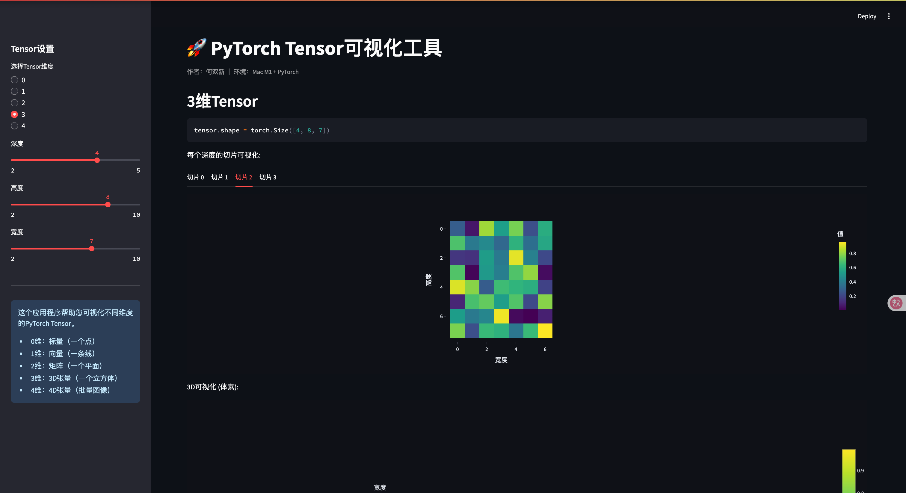
elif tensor_dim == 3: # 3D Tensor
depth = st.sidebar.slider("深度", 2, 5, 3)
height = st.sidebar.slider("高度", 2, 10, 5)
width = st.sidebar.slider("宽度", 2, 10, 5)
st.header("3维Tensor")
tensor = torch.rand(depth, height, width)
st.code(f"tensor.shape = {tensor.shape}")
# 展示每个深度层
st.write("每个深度的切片可视化:")
tabs = st.tabs([f"切片 {i}" for i in range(depth)])
for i, tab in enumerate(tabs):
with tab:
fig = px.imshow(tensor[i].numpy(),
labels=dict(x="宽度", y="高度", color="值"),
color_continuous_scale='viridis')
fig.update_layout(width=500, height=400)
st.plotly_chart(fig)
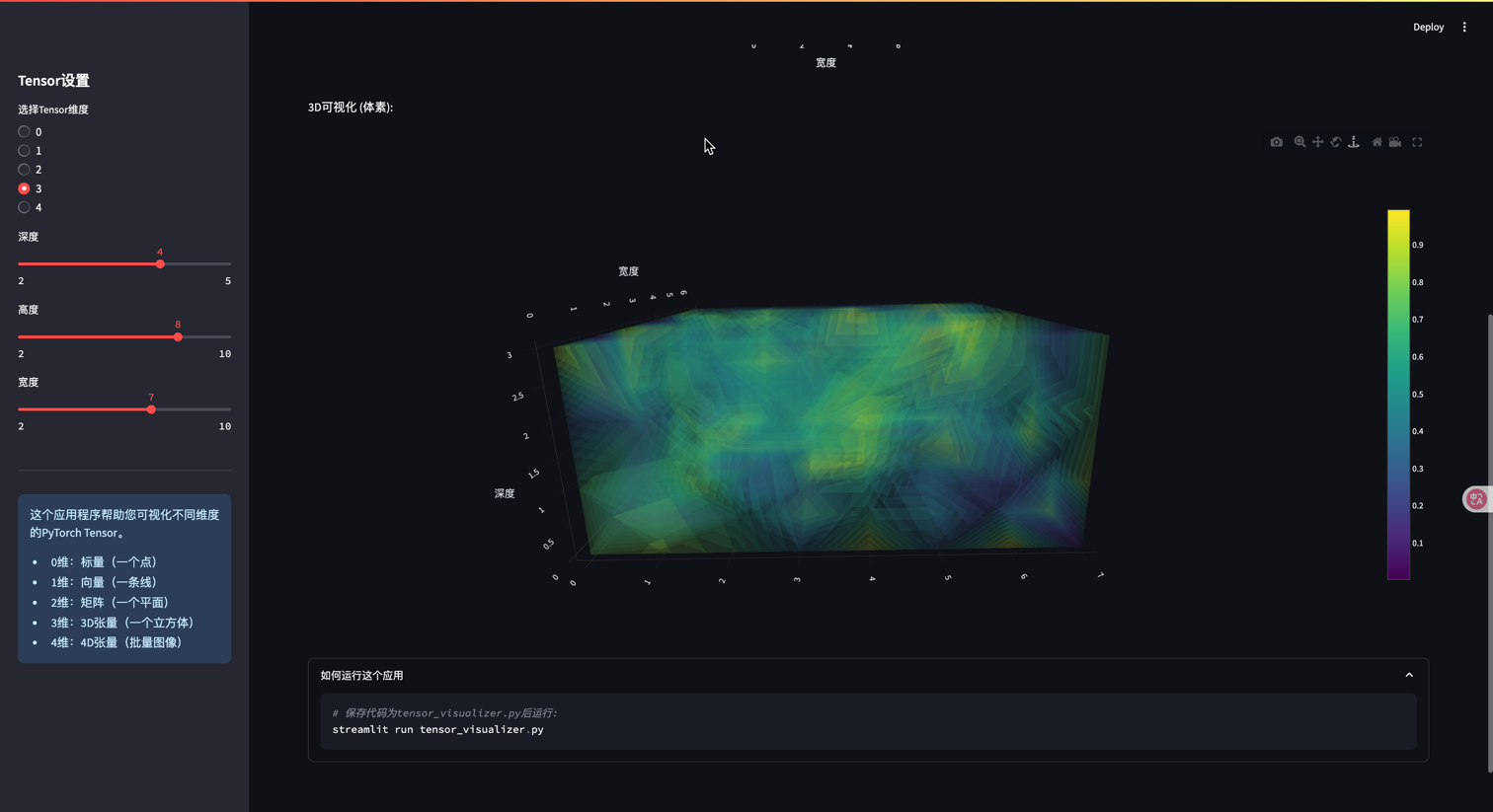
# 3D可视化
st.write("3D可视化 (体素):")
# 创建网格
X, Y, Z = np.mgrid[0:depth, 0:height, 0:width]
values = tensor.numpy().flatten()
fig = go.Figure(data=go.Volume(
x=X.flatten(),
y=Y.flatten(),
z=Z.flatten(),
value=values,
opacity=0.1,
surface_count=15,
colorscale='viridis'
))
fig.update_layout(
scene=dict(xaxis_title='深度', yaxis_title='高度', zaxis_title='宽度'),
width=700, height=700
)
st.plotly_chart(fig)
elif tensor_dim == 4: # 4D Tensor
batch = st.sidebar.slider("批量大小", 1, 5, 2)
channels = st.sidebar.slider("通道数", 1, 3, 3)
height = st.sidebar.slider("高度", 4, 12, 8)
width = st.sidebar.slider("宽度", 4, 12, 8)
st.header("4维Tensor (批量图像)")
tensor = torch.rand(batch, channels, height, width)
st.code(f"tensor.shape = {tensor.shape}")
st.write(f"这个Tensor可以表示{batch}张{channels}通道的{height}x{width}图像")
# 可视化每个批次的图像
batch_tabs = st.tabs([f"批次 {i}" for i in range(batch)])
for b, batch_tab in enumerate(batch_tabs):
with batch_tab:
if channels == 3:
# 针对RGB图像的特殊处理
img = tensor[b].permute(1, 2, 0).numpy() # 转换为HWC格式
st.image(img, caption=f"批次 {b} 的RGB图像", use_column_width=True)
else:
# 展示每个通道
channel_tabs = st.tabs([f"通道 {i}" for i in range(channels)])
for c, channel_tab in enumerate(channel_tabs):
with channel_tab:
fig = px.imshow(tensor[b, c].numpy(),
color_continuous_scale='viridis')
fig.update_layout(width=400, height=400)
st.plotly_chart(fig)
# 添加信息部分
st.sidebar.markdown("---")
st.sidebar.info("""
这个应用程序帮助您可视化不同维度的PyTorch Tensor。
- 0维:标量(一个点)
- 1维:向量(一条线)
- 2维:矩阵(一个平面)
- 3维:3D张量(一个立方体)
- 4维:4D张量(批量图像)
""")
# 添加代码说明
with st.expander("如何运行这个应用"):
st.code("""
# 保存代码为tensor_visualizer.py后运行:
streamlit run tensor_visualizer.py
""")
7. 总结
在本篇博客中,我们深入探讨了PyTorch中的两个核心概念:
- Tensor广播机制 - 使不同形状的张量能够进行运算,避免不必要的内存复制,提高代码效率
- 自动求导机制 - 自动构建计算图并执行反向传播,计算各参数的梯度,是深度学习优化的基础