生成模型实战 | GLOW详解与实现
-
- [0. 前言](#0. 前言)
- [1. 归一化流模型](#1. 归一化流模型)
-
- [1.1 归一化流与变换公式](#1.1 归一化流与变换公式)
- [1.2 RealNVP 的通道翻转](#1.2 RealNVP 的通道翻转)
- [2. GLOW 架构](#2. GLOW 架构)
-
- [2.1 ActNorm](#2.1 ActNorm)
- [2.2 可逆 1×1 卷积](#2.2 可逆 1×1 卷积)
- [2.3 仿射耦合层](#2.3 仿射耦合层)
- [2.4 多尺度架构](#2.4 多尺度架构)
- [3. 使用 PyTorch 实现 GLOW](#3. 使用 PyTorch 实现 GLOW)
-
- [3.1 数据处理](#3.1 数据处理)
- [3.2 模型构建](#3.2 模型构建)
- [3.3 模型训练](#3.3 模型训练)
0. 前言
GLOW (Generative Flow) 是一种基于归一化流的生成模型,通过在每个流步骤中引入可逆的 1 × 1 卷积层,替代了RealNVP中通道翻转或固定置换的策略,从而使通道重排更具表达力,同时保持雅可比行列式和逆变换的高效计算能力。本文首先回顾归一化流与 RealNVP 的基本原理,接着剖析 GLOW 的四大核心模块:ActNorm、可逆 1×1 卷积、仿射耦合层和多尺度架构,随后基于 PyTorch 实现 GLOW 模型,并在 CIFAR-10 数据集上进行训练。
1. 归一化流模型
1.1 归一化流与变换公式
在本节中,我们首先简要回顾归一化流模型的核心原理,归一化流利用可逆映射 f f f 将简单分布 p Z ( z ) p_Z(z) pZ(z) 转换到样本分布 p X ( x ) p_X(x) pX(x),并通过以下变换公式实现实现精确对数似然计算和采样:
p X ( x ) = p Z ( f ( x ) ) ∣ det ( ∂ f ( x ) ∂ x ) ∣ p_X(x)=p_Z(f(x)) |\text{det} (\frac {∂f(x)}{∂x})| pX(x)=pZ(f(x)) ∣det(∂x∂f(x))∣
1.2 RealNVP 的通道翻转
RealNVP 通过交替使用掩码耦合层 (masking coupling) 和按通道翻转 (reverse channels) 或固定置换,保证每个通道都能被多次变换。
2. GLOW 架构
2.1 ActNorm
ActNorm 是一种专为流模型设计的通道级归一化方法,于 GLOW 中首次提出。该层对输入激活 x x x 执行可学习仿射变换:
y = s ⊙ x + b y=s⊙x+b y=s⊙x+b
其中 s , b ∈ R C s,b∈\mathbb R^C s,b∈RC 分别为每个通道的尺度与偏移参数。这些参数在首次前向传播时通过对一个 minibatch 计算输出通道的均值 μ μ μ 和标准差 σ σ σ 进行数据依赖的初始化,使得初始化后的 y y y 满足 E y = 0 \mathbb Ey=0 Ey=0 和 V a r y = 1 Vary=1 Vary=1。
与批归一化不同,ActNorm 仅在初始化时依赖 minibatch,之后无需维护运行时统计量,从而提升了小批数据和解耦训练的稳定性。
python
import torch.nn as nn
import torch

def mean_dim(tensor, dim=None, keepdims=False):
    if dim is None:
        return tensor.mean()
    else:
        if isinstance(dim, int):
            dim = [dim]
        dim = sorted(dim)
        for d in dim:
            tensor = tensor.mean(dim=d, keepdim=True)
        if not keepdims:
            for i, d in enumerate(dim):
                tensor.squeeze_(d-i)
        return tensor

class ActNorm(nn.Module):
    def __init__(self, num_features, scale=1., return_ldj=False):
        super(ActNorm, self).__init__()
        self.register_buffer('is_initialized', torch.zeros(1))
        self.bias = nn.Parameter(torch.zeros(1, num_features, 1, 1))
        self.logs = nn.Parameter(torch.zeros(1, num_features, 1, 1))

        self.num_features = num_features
        self.scale = float(scale)
        self.eps = 1e-6
        self.return_ldj = return_ldj

    def initialize_parameters(self, x):
        if not self.training:
            return

        with torch.no_grad():
            bias = -mean_dim(x.clone(), dim=[0, 2, 3], keepdims=True)
            v = mean_dim((x.clone() + bias) ** 2, dim=[0, 2, 3], keepdims=True)
            logs = (self.scale / (v.sqrt() + self.eps)).log()
            self.bias.data.copy_(bias.data)
            self.logs.data.copy_(logs.data)
            self.is_initialized += 1.

    def _center(self, x, reverse=False):
        if reverse:
            return x - self.bias
        else:
            return x + self.bias

    def _scale(self, x, sldj, reverse=False):
        logs = self.logs
        if reverse:
            x = x * logs.mul(-1).exp()
        else:
            x = x * logs.exp()

        if sldj is not None:
            ldj = logs.sum() * x.size(2) * x.size(3)
            if reverse:
                sldj = sldj - ldj
            else:
                sldj = sldj + ldj

        return x, sldj

    def forward(self, x, ldj=None, reverse=False):
        if not self.is_initialized:
            self.initialize_parameters(x)

        if reverse:
            x, ldj = self._scale(x, ldj, reverse)
            x = self._center(x, reverse)
        else:
            x = self._center(x, reverse)
            x, ldj = self._scale(x, ldj, reverse)

        if self.return_ldj:
            return x, ldj

        return x
2.2 可逆 1×1 卷积
GLOW 中的可逆 1×1 卷积用一个 C × C C×C C×C 的可学习矩阵 W W W 取代了 RealNVP 中的固定通道翻转或置换操作。在空间位置 ( i , j ) (i,j) (i,j) 上,其映射可写为:
y i , j = W x i , j y_{i,j}=W x_{i,j} yi,j=W xi,j
对应的对数行列式为:
log det ∣ ∂ y ∂ x ∣ = H × W × log ∣ det W ∣ \text {log}\ \text{det} |\frac{∂y}{∂x}|=H×W×\text {log}|\text{det}W| log det ∣∂x∂y∣=H×W×log∣detW∣
其中 H , W H,W H,W 分别为空间高宽。
为了进一步加速行列式与逆矩阵的计算,通常将 W W W 参数化为 LU 分解形式,即 W = P L U W=PLU W=PLU,只需学习下三角矩阵 L L L 和上三角矩阵 U U U 的非对角元素,行列式则为 ∏ i U i i ∏iU{ii} ∏iUii。
通过这种可学习的通道重排,模型能够自动挖掘最优的特征混合方式,从而在生成质量与训练效率上均取得显著提升。
python
import numpy as np

class InvConv(nn.Module):
    def __init__(self, num_channels):
        super(InvConv, self).__init__()
        self.num_channels = num_channels

        # Initialize with a random orthogonal matrix
        w_init = np.random.randn(num_channels, num_channels)
        w_init = np.linalg.qr(w_init)[0].astype(np.float32)
        self.weight = nn.Parameter(torch.from_numpy(w_init))

    def forward(self, x, sldj, reverse=False):
        ldj = torch.slogdet(self.weight)[1] * x.size(2) * x.size(3)

        if reverse:
            weight = torch.inverse(self.weight.double()).float()
            sldj = sldj - ldj
        else:
            weight = self.weight
            sldj = sldj + ldj

        weight = weight.view(self.num_channels, self.num_channels, 1, 1)
        z = F.conv2d(x, weight)

        return z, sldj
2.3 仿射耦合层
仿射耦合层最早在 RealNVP 中提出,是 GLOW 中不可或缺的组成部分。该层将输入 x ∈ R C × H × W x∈\mathbb R^{C×H×W} x∈RC×H×W 沿通道维度划分为两部分 ( x a , x b ) (x_a,x_b) (xa,xb),并通过神经网络生成尺度和平移参数保证了整个变换的可逆性:
( s , t ) = N N ( x b ) , y a = s ( x b ) ⊙ x a + t ( x b ) , y b = x b (s,t)=NN(x_b),ya=s(x_b)⊙x_a+t(x_b),y_b=x_b (s,t)=NN(xb),ya=s(xb)⊙xa+t(xb),yb=xb
其对数雅可比行列式可高效地计算为:
∑ h , w , c ∈ a log s c ( x b h , w ) ∑_{h,w, c∈a}\text {log}s_c(x_bh,w) h,w, c∈a∑logsc(xbh,w)
仅与输出尺度参数 s s s 的元素相加相关,计算复杂度随输入维度线性增长。
python
import torch.nn.functional as F

class Coupling(nn.Module):
    def __init__(self, in_channels, mid_channels):
        super(Coupling, self).__init__()
        self.nn = NN(in_channels, mid_channels, 2 * in_channels)
        self.scale = nn.Parameter(torch.ones(in_channels, 1, 1))

    def forward(self, x, ldj, reverse=False):
        x_change, x_id = x.chunk(2, dim=1)

        st = self.nn(x_id)
        s, t = st[:, 0::2, ...], st[:, 1::2, ...]
        s = self.scale * torch.tanh(s)

        # Scale and translate
        if reverse:
            x_change = x_change * s.mul(-1).exp() - t
            ldj = ldj - s.flatten(1).sum(-1)
        else:
            x_change = (x_change + t) * s.exp()
            ldj = ldj + s.flatten(1).sum(-1)

        x = torch.cat((x_change, x_id), dim=1)

        return x, ldj


class NN(nn.Module):
    def __init__(self, in_channels, mid_channels, out_channels,
                 use_act_norm=False):
        super(NN, self).__init__()
        norm_fn = ActNorm if use_act_norm else nn.BatchNorm2d

        self.in_norm = norm_fn(in_channels)
        self.in_conv = nn.Conv2d(in_channels, mid_channels,
                                 kernel_size=3, padding=1, bias=False)
        nn.init.normal_(self.in_conv.weight, 0., 0.05)

        self.mid_norm = norm_fn(mid_channels)
        self.mid_conv = nn.Conv2d(mid_channels, mid_channels,
                                  kernel_size=1, padding=0, bias=False)
        nn.init.normal_(self.mid_conv.weight, 0., 0.05)

        self.out_norm = norm_fn(mid_channels)
        self.out_conv = nn.Conv2d(mid_channels, out_channels,
                                  kernel_size=3, padding=1, bias=True)
        nn.init.zeros_(self.out_conv.weight)
        nn.init.zeros_(self.out_conv.bias)

    def forward(self, x):
        x = self.in_norm(x)
        x = F.relu(x)
        x = self.in_conv(x)

        x = self.mid_norm(x)
        x = F.relu(x)
        x = self.mid_conv(x)

        x = self.out_norm(x)
        x = F.relu(x)
        x = self.out_conv(x)

        return x
2.4 多尺度架构
GLOW 延续了 RealNVP 的多尺度架构思想,通过分层的流步骤和因子化操作将中间表示逐级分解。整体模型由 L L L 个尺度 (level) 组成,每个尺度内部包含 K K K 次完整的流步骤 (step),每步依次执行 ActNorm、可逆 1×1 卷积和仿射耦合层。
在每个尺度结束时,先通过 squeeze 操作将特征图空间大小减少至原像素的四分之一(同时通道数扩大四倍),然后使用 split 操作将部分通道因子化为潜变量 z z z,余下通道继续进入下一级流。
这种多尺度分解在保持对数似然精度的同时,有效降低了计算与存储开销,并在不同尺度上捕捉图像的全局与局部结构信息。
3. 使用 PyTorch 实现 GLOW
在本节中,使用 PyTorch 实现 GLOW,并在 CIFAR-10 数据集上进行训练。
3.1 数据处理
用 torchvision.transforms 对 CIFAR-10 图像进行处理:
python
transform_train = transforms.Compose([
        transforms.RandomHorizontalFlip(),
        transforms.ToTensor()
    ])

transform_test = transforms.Compose([
    transforms.ToTensor()
])

trainset = torchvision.datasets.CIFAR10(root='data', train=True, download=True, transform=transform_train)
trainloader = data.DataLoader(trainset, batch_size=batch_size, shuffle=True, num_workers=num_workers)

testset = torchvision.datasets.CIFAR10(root='data', train=False, download=True, transform=transform_test)
testloader = data.DataLoader(testset, batch_size=batch_size, shuffle=False, num_workers=num_workers)
3.2 模型构建
基于 ActNorm、可逆 1×1 卷积、仿射耦合层和多尺度架构实现 GLOW 模型:
python
class Glow(nn.Module):
    def __init__(self, num_channels, num_levels, num_steps):
        super(Glow, self).__init__()

        # Use bounds to rescale images before converting to logits, not learned
        self.register_buffer('bounds', torch.tensor([0.9], dtype=torch.float32))
        self.flows = _Glow(in_channels=4 * 3,  # RGB image after squeeze
                           mid_channels=num_channels,
                           num_levels=num_levels,
                           num_steps=num_steps)

    def forward(self, x, reverse=False):
        if reverse:
            sldj = torch.zeros(x.size(0), device=x.device)
        else:
            # Expect inputs in [0, 1]
            if x.min() < 0 or x.max() > 1:
                raise ValueError('Expected x in [0, 1], got min/max {}/{}'
                                 .format(x.min(), x.max()))

            # De-quantize and convert to logits
            x, sldj = self._pre_process(x)

        x = squeeze(x)
        x, sldj = self.flows(x, sldj, reverse)
        x = squeeze(x, reverse=True)

        return x, sldj

    def _pre_process(self, x):
        y = (x * 255. + torch.rand_like(x)) / 256.
        y = (2 * y - 1) * self.bounds
        y = (y + 1) / 2
        y = y.log() - (1. - y).log()

        # Save log-determinant of Jacobian of initial transform
        ldj = F.softplus(y) + F.softplus(-y) \
            - F.softplus((1. - self.bounds).log() - self.bounds.log())
        sldj = ldj.flatten(1).sum(-1)

        return y, sldj

class _Glow(nn.Module):
    def __init__(self, in_channels, mid_channels, num_levels, num_steps):
        super(_Glow, self).__init__()
        self.steps = nn.ModuleList([_FlowStep(in_channels=in_channels,
                                              mid_channels=mid_channels)
                                    for _ in range(num_steps)])

        if num_levels > 1:
            self.next = _Glow(in_channels=2 * in_channels,
                              mid_channels=mid_channels,
                              num_levels=num_levels - 1,
                              num_steps=num_steps)
        else:
            self.next = None

    def forward(self, x, sldj, reverse=False):
        if not reverse:
            for step in self.steps:
                x, sldj = step(x, sldj, reverse)

        if self.next is not None:
            x = squeeze(x)
            x, x_split = x.chunk(2, dim=1)
            x, sldj = self.next(x, sldj, reverse)
            x = torch.cat((x, x_split), dim=1)
            x = squeeze(x, reverse=True)

        if reverse:
            for step in reversed(self.steps):
                x, sldj = step(x, sldj, reverse)

        return x, sldj


class _FlowStep(nn.Module):
    def __init__(self, in_channels, mid_channels):
        super(_FlowStep, self).__init__()
        # Activation normalization, invertible 1x1 convolution, affine coupling
        self.norm = ActNorm(in_channels, return_ldj=True)
        self.conv = InvConv(in_channels)
        self.coup = Coupling(in_channels // 2, mid_channels)

    def forward(self, x, sldj=None, reverse=False):
        if reverse:
            x, sldj = self.coup(x, sldj, reverse)
            x, sldj = self.conv(x, sldj, reverse)
            x, sldj = self.norm(x, sldj, reverse)
        else:
            x, sldj = self.norm(x, sldj, reverse)
            x, sldj = self.conv(x, sldj, reverse)
            x, sldj = self.coup(x, sldj, reverse)

        return x, sldj


def squeeze(x, reverse=False):
    b, c, h, w = x.size()
    if reverse:
        # Unsqueeze
        x = x.view(b, c // 4, 2, 2, h, w)
        x = x.permute(0, 1, 4, 2, 5, 3).contiguous()
        x = x.view(b, c // 4, h * 2, w * 2)
    else:
        # Squeeze
        x = x.view(b, c, h // 2, 2, w // 2, 2)
        x = x.permute(0, 1, 3, 5, 2, 4).contiguous()
        x = x.view(b, c * 2 * 2, h // 2, w // 2)

    return x
3.3 模型训练
实例化模型、损失函数和优化器,并进行训练:
python
net = Glow(num_channels=num_channels,
num_levels=num_levels,
num_steps=num_steps)
net = net.to(device)
loss_fn = NLLLoss().to(device)
optimizer = optim.Adam(net.parameters(), lr=lr)
scheduler = sched.LambdaLR(optimizer, lambda s: min(1., s / warm_up))
@torch.enable_grad()
def train(epoch, net, trainloader, device, optimizer, scheduler, loss_fn, max_grad_norm):
global global_step
print('\nEpoch: %d' % epoch)
net.train()
loss_meter = AverageMeter()
with tqdm(total=len(trainloader.dataset)) as progress_bar:
for x, _ in trainloader:
x = x.to(device)
optimizer.zero_grad()
z, sldj = net(x, reverse=False)
loss = loss_fn(z, sldj)
loss_meter.update(loss.item(), x.size(0))
loss.backward()
if max_grad_norm > 0:
clip_grad_norm(optimizer, max_grad_norm)
optimizer.step()
scheduler.step(global_step)
progress_bar.set_postfix(nll=loss_meter.avg,
bpd=bits_per_dim(x, loss_meter.avg),
lr=optimizer.param_groups[0]['lr'])
progress_bar.update(x.size(0))
global_step += x.size(0)
@torch.no_grad()
def sample(net, batch_size, device):
z = torch.randn((batch_size, 3, 32, 32), dtype=torch.float32, device=device)
x, _ = net(z, reverse=True)
x = torch.sigmoid(x)
return x
@torch.no_grad()
def test(epoch, net, testloader, device, loss_fn, num_samples):
global best_loss
net.eval()
loss_meter = AverageMeter()
with tqdm(total=len(testloader.dataset)) as progress_bar:
for x, _ in testloader:
x = x.to(device)
z, sldj = net(x, reverse=False)
loss = loss_fn(z, sldj)
loss_meter.update(loss.item(), x.size(0))
progress_bar.set_postfix(nll=loss_meter.avg,
bpd=bits_per_dim(x, loss_meter.avg))
progress_bar.update(x.size(0))
# Save checkpoint
if loss_meter.avg < best_loss:
print('Saving...')
state = {
'net': net.state_dict(),
'test_loss': loss_meter.avg,
'epoch': epoch,
}
os.makedirs('ckpts', exist_ok=True)
torch.save(state, 'ckpts/best.pth.tar')
best_loss = loss_meter.avg
# Save samples and data
images = sample(net, num_samples, device)
os.makedirs('samples', exist_ok=True)
images_concat = torchvision.utils.make_grid(images, nrow=int(num_samples ** 0.5), padding=2, pad_value=255)
torchvision.utils.save_image(images_concat, 'samples/epoch_{}.png'.format(epoch))
start_epoch = 0
for epoch in range(start_epoch, start_epoch + num_epochs):
train(epoch, net, trainloader, device, optimizer, scheduler,
loss_fn, max_grad_norm)
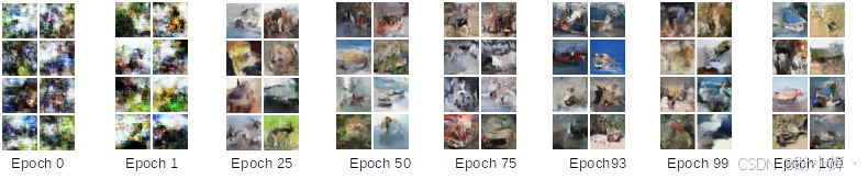
test(epoch, net, testloader, device, loss_fn, num_samples)在 100 个 epoch 后,模型可生成逼真度较高的 32 × 32 彩色图像,样本在多通道细节和整体结构上均有良好效果,下图展示了训练过程中,不同 epoch 生成的图像对比: